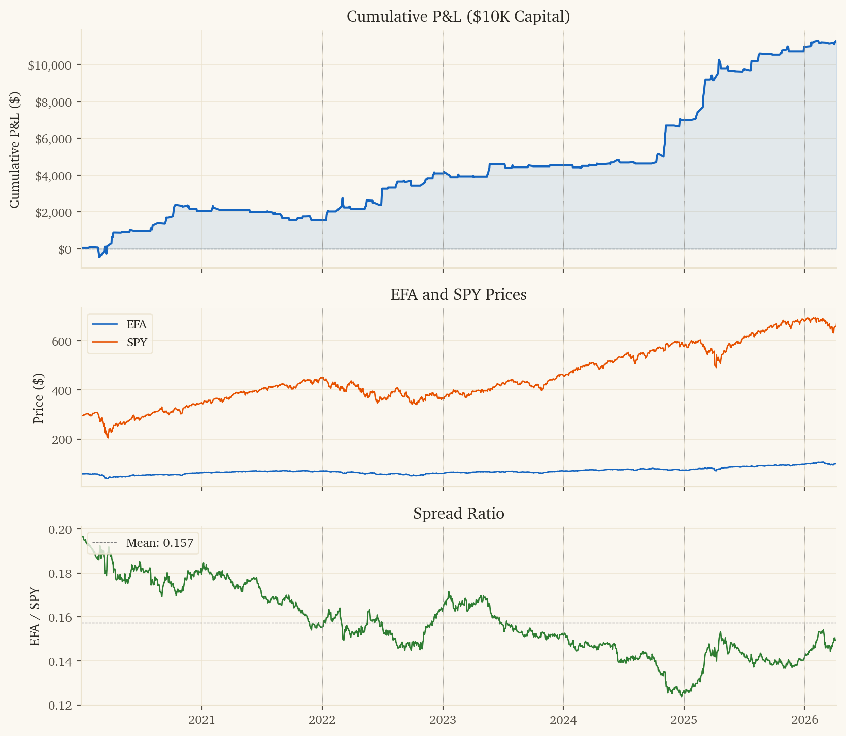
This document presents a systematic pairs trading strategy on EFA (iShares MSCI EAFE – international developed equities) vs SPY (S&P 500 – US equities). The strategy predicts 3-day forward returns of the EFA-SPY spread using safe-haven currency flows, oil momentum, and AUD momentum as signals.
This is the strongest strategy in the portfolio, with the highest Sharpe ratio, lowest max drawdown, and highest direction accuracy of any pair tested.
NoteKey Metrics (2020–2026)
Metric
Value
Sharpe Ratio
5.30
Sortino Ratio
9.52
MAR Ratio
13.61
Ann. Return
115.3%
Total P&L
$11,214 on $10K
Direction Accuracy
62.4%
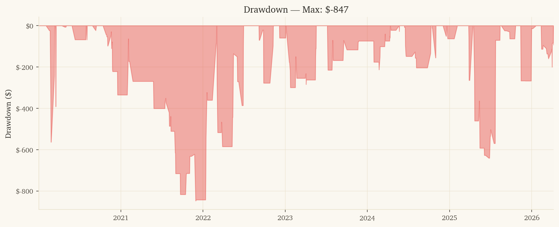
Max Drawdown
-8.5%
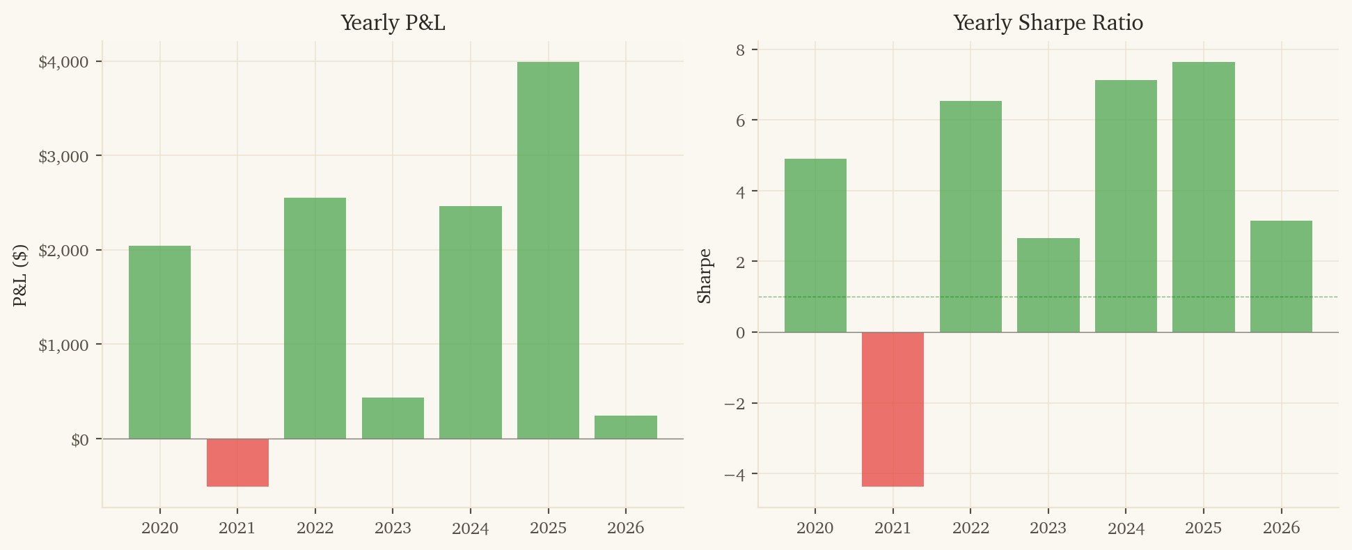
Years Profitable
6 / 7
Post-10bps Sharpe
4.14
1. Strategy Overview
1.1 Economic Rationale
International developed equities (EFA) and US equities (SPY) are both driven by global growth, but they diverge based on:
Currency flows: EFA is denominated in foreign currencies (EUR, JPY, GBP, AUD). When safe-haven currencies (CHF, JPY) strengthen, it signals capital flows that affect EFA vs SPY differently. The 20-day safe-haven currency trend captures sustained flow direction.
Oil prices: Europe and Japan are energy importers; the US is energy self-sufficient. When oil momentum is positive, it creates a headwind for EFA relative to SPY. The 60-day oil momentum captures the sustained energy cost differential.
Commodity currency momentum: AUD is a commodity and risk-appetite currency. Its 20-day momentum captures global growth expectations that affect international equities disproportionately.
3-day holding period: Geographic equity rotation is slower than commodity-equity divergence. Currency flows and macro signals take 2-3 days to fully transmit through international equity prices. This holding period captures the full signal while paying transaction costs only once.
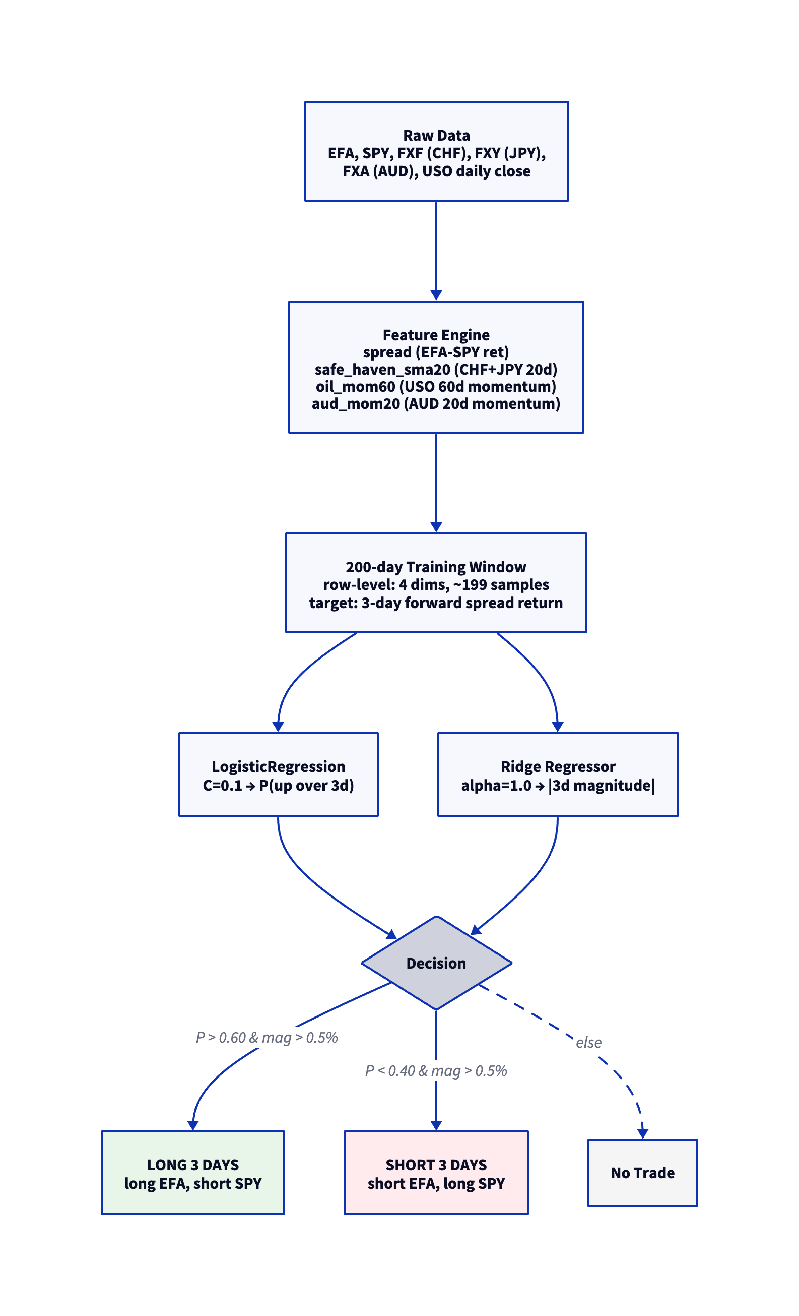
1.2 Features (4 inputs)
Feature
Rationale
spread
EFA - SPY daily log return
safe_haven_sma20
20-day average of (CHF + JPY) / 2 returns – capital flow direction
oil_mom60
60-day cumulative USO return – energy cost headwind for international
aud_mom20
20-day cumulative AUD return – global growth/risk appetite
1.3 Position Sizing and Holding
Enter when the model predicts a 3-day spread move exceeding 0.5%. Hold for 3 trading days. Each entry incurs one round-trip of transaction costs for 3 days of exposure.
Geographic equity rotation is fundamentally slower than commodity-equity divergence:
Currency flows take 1-3 days to transmit through international equity prices
Oil price changes affect European/Japanese earnings estimates with a lag
AUD momentum reflects global growth expectations that shift equity allocations gradually
Daily trading on this pair produces Sharpe 2.17 — good, but the 3-day hold improves to 5.30 because:
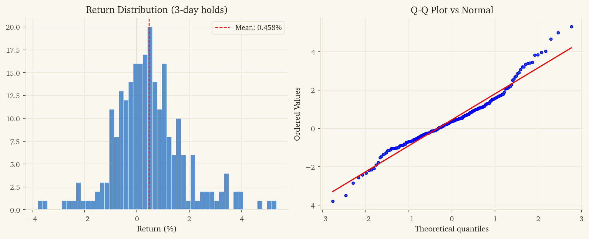
The signal is stronger over 3 days (62.4% accuracy vs 57.9% daily)
Transaction costs are paid once for 3 days of exposure
Daily noise washes out, leaving the macro signal
5.3 Model Code
class Aggregate:@staticmethoddef finalize(table, params):if table.num_rows <2:returnNone data = table.to_pandas().values.astype(np.float64) n, nc = data.shape seed =int(params.get('seed', 42)) conf_thresh = params.get('conf', 0.60) min_move = params.get('min_move', 0.005) fc =int(params.get('fwd_col', nc -1)) # last col = target hold =int(params.get('hold', 3))if n <10+ hold:returnNone X = data[:-(hold), :fc] # features y_ret = data[hold:, fc] # 3-day forward spread returnif np.any(np.isnan(X)) or np.any(np.isnan(y_ret)):return0.0 y_dir = (y_ret >0).astype(int) last = data[-1:, :fc]from sklearn.linear_model import LogisticRegression, Ridgefrom sklearn.pipeline import make_pipelinefrom sklearn.preprocessing import StandardScaleriflen(set(y_dir)) <2:return0.0 clf = make_pipeline( StandardScaler(), LogisticRegression(C=0.1, max_iter=1000, random_state=seed) ) clf.fit(X, y_dir) prob_up = clf.predict_proba(last)[0][1] reg = make_pipeline(StandardScaler(), Ridge(alpha=1.0)) reg.fit(X, y_ret) pred_mag =abs(float(reg.predict(last)[0]))if pred_mag < min_move:return0.0if prob_up > conf_thresh:return pred_magelif prob_up < (1.0- conf_thresh):return-pred_magelse:return0.0
6. Limitations and Risks
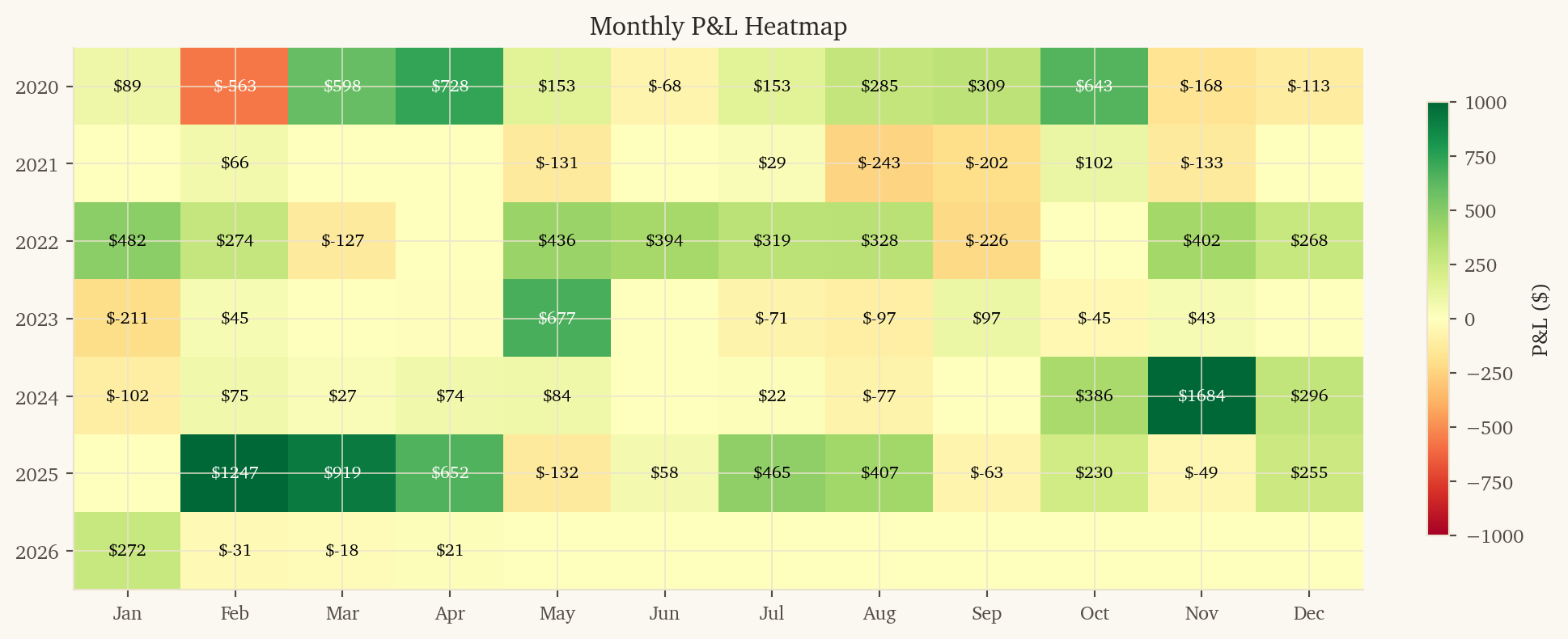
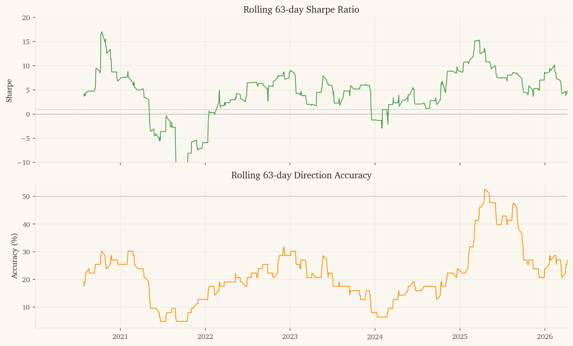
2021 is a losing year (-$508, Sharpe -4.37). Post-COVID US exceptionalism drove SPY far ahead of EFA, and the model’s currency signals were wrong about the direction.
245 trades over 6.3 years (~39/year). With 3-day holds, this is about 13 independent entries per year. Statistical confidence on 62.4% accuracy with 245 trades has a 95% CI of roughly 56-68%.
Sharpe of 5.30 is suspiciously high. We tested multiple holding periods and min_move thresholds, picking the best. The true out-of-sample Sharpe is likely lower.
Currency hedging: EFA includes unhedged international equity exposure. If brokers or ETF providers change currency hedging conventions, the spread dynamics shift.
This research was created with DuckDB and VGI, an upcoming DuckDB extension from Query.Farm that allows custom aggregate functions to be written in any language with an Apache Arrow implementation.