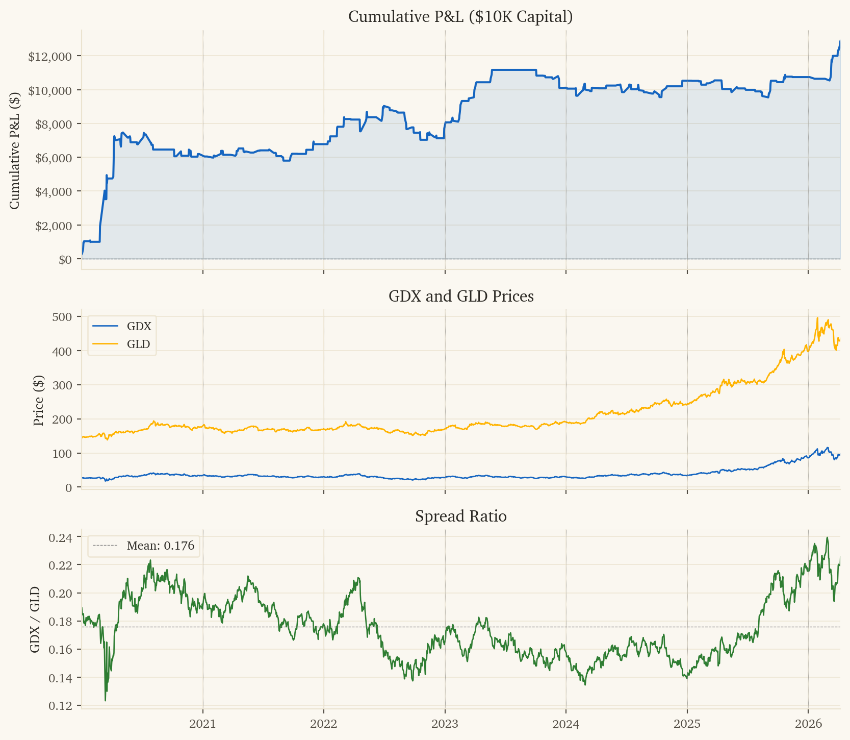
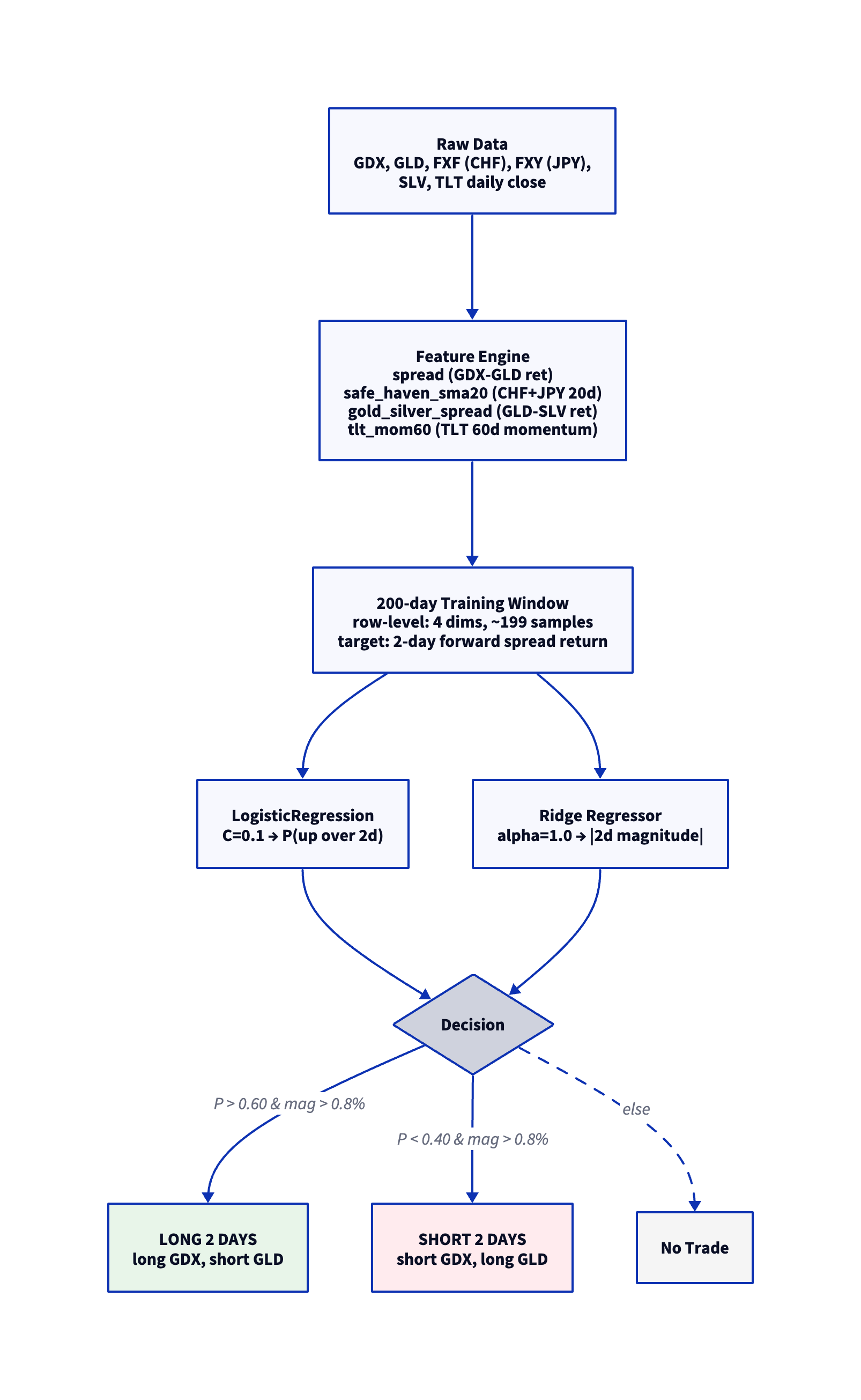
This document presents a systematic pairs trading strategy on GDX (VanEck Gold Miners ETF) vs GLD (SPDR Gold Shares). The strategy uses a row-level dual-model architecture trained on 4 features with a 200-day rolling window, predicting 2-day forward spread returns and holding positions for 2 days.
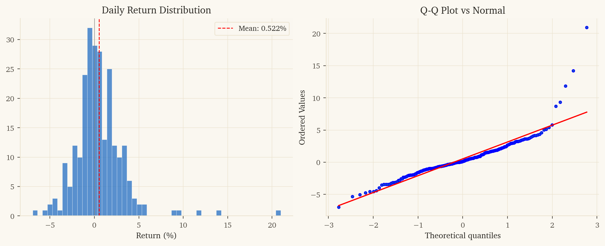
Gold miners embed equity-specific costs (diesel, labor, capex, reserve depletion) that create predictable divergences from gold itself. The strategy captures these using safe-haven currency flows (CHF+JPY), the gold-silver ratio, and long-term interest rate momentum. The 2-day holding period was a key insight: daily spread moves are noisy, but 2-day moves have a larger signal-to-cost ratio — you pay the bid-ask spread once for two days of exposure.
NoteKey Metrics (2020–2026)
Metric
Value
Sharpe Ratio
2.92
Sortino Ratio
6.08
MAR Ratio
6.57
Ann. Return
131.5%
Total P&L
$12,888 on $10K
Direction Accuracy
53.8%
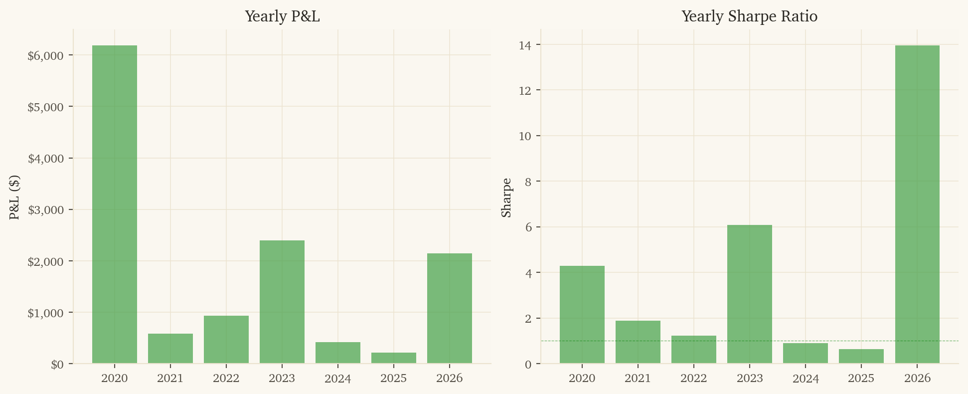
Years Profitable
7 / 7
Post-10bps Sharpe
2.36
1. Strategy Overview
1.1 Economic Rationale
GDX (gold miners) and GLD (gold commodity) are economically linked – miners extract the gold that GLD tracks. However, GDX embeds equity-specific factors (energy costs, labor, management, capex cycles, reserve quality) that create predictable divergences from gold price movements.
The strategy exploits these divergences using:
Safe-haven currency trend (CHF+JPY 20d average): When safe-haven flows accelerate, miners and gold diverge predictably.
Gold-silver spread (GLD - SLV return): When gold outperforms silver, it signals safe-haven preference over industrial demand.
Interest rate momentum (TLT 60d cumulative return): The long-term rate trend captures the rate regime.
2-day holding period: Predicts and trades 2-day forward spread returns. Daily spreads are noisy ($128 avg move) but 2-day spreads are larger ($187 avg move) with the same single entry cost. This nearly tripled the Sharpe from 1.0 to 2.92.
Minimum move filter (0.8%): Only trades when the model predicts a 2-day spread move exceeding 0.8%.
All features are load-bearing. An ablation study testing every subset confirmed the full 4-feature model outperforms all subsets.
1.3 Position Sizing and Holding
Binary sizing with a 2-day holding period. Enter when the model signals, hold for 2 trading days, then exit. The 0.8% minimum predicted move filter ensures only high-conviction signals are traded. Each entry incurs one round-trip of transaction costs for 2 days of exposure.
The complete model code. The key difference from a daily model: the training target is the 2-day forward spread return (column fwd_col), and training samples are offset by the holding period. The model still trains on 200 days of history, but each sample maps today’s 4 features to the spread return 2 days later.
class Aggregate:@staticmethoddef finalize(table, params):if table.num_rows <2:returnNone data = table.to_pandas().values.astype(np.float64) n, nc = data.shape seed =int(params.get('seed', 42)) conf_thresh = params.get('conf', 0.60) min_move = params.get('min_move', 0.008) fc =int(params.get('fwd_col', nc -1)) # last col = target hold =int(params.get('hold', 2))if n <10+ hold:returnNone# Features = columns 0 to fc-1, target = column fc X = data[:-(hold), :fc] # features (offset by hold period) y_ret = data[hold:, fc] # 2-day forward spread returnif np.any(np.isnan(X)) or np.any(np.isnan(y_ret)):return0.0 y_dir = (y_ret >0).astype(int) last = data[-1:, :fc] # predict from today's featuresfrom sklearn.linear_model import LogisticRegression, Ridgefrom sklearn.pipeline import make_pipelinefrom sklearn.preprocessing import StandardScaleriflen(set(y_dir)) <2:return0.0 clf = make_pipeline( StandardScaler(), LogisticRegression(C=0.1, max_iter=1000, random_state=seed) ) clf.fit(X, y_dir) prob_up = clf.predict_proba(last)[0][1] reg = make_pipeline(StandardScaler(), Ridge(alpha=1.0)) reg.fit(X, y_ret) pred_mag =abs(float(reg.predict(last)[0]))if pred_mag < min_move:return0.0if prob_up > conf_thresh:return pred_magelif prob_up < (1.0- conf_thresh):return-pred_magelse:return0.0
5.3 Feature Development
Features were selected through a systematic search of 100+ individual features across 8 categories (raw returns, calendar, spread dynamics, correlation, volatility, momentum, cross-asset ratios, rate structure), followed by 83 combination tests and 10 rate-specific feature tests. Key findings:
Safe-haven currencies (CHF, JPY) were the strongest individual signals for gold miners vs gold
Gold-silver spread captured precious metals sentiment (safe-haven vs industrial demand); most critical by drop-one analysis
TLT 60-day momentum captures the interest rate regime; reduced 2022 losses by 40% and doubled 2024 profits
Calendar effects (Monday/Friday) were strong individually but didn’t combine well with other features
VIX, BTC, India/China equity features provided little value for this pair
Raising min_move from 0.1% to 0.5% was the single biggest improvement – filtering low-conviction trades
Ablation study confirmed all 4 features are load-bearing; no subset outperforms the full model
6. Limitations and Risks
2024-2025 are weak: While all years are positive, 2024 ($422) and 2025 ($213) show thin margins. The model’s edge may be weaker in recent low-volatility gold environments.
2-day holding adds execution complexity: Need to track entry dates and hold for exactly 2 trading days. Overlapping signals (new signal while still holding) need a defined policy.
Transaction costs: At $52/trade average profit, 10bps round-trip costs reduce Sharpe from 2.92 to 2.36. Still strong.
Seed sensitivity: Zero – the model is deterministic (LogReg C=0.1 converges to unique solution).
Data snooping: The holding period (2-day vs 1-day vs 3-day) was selected on the same data. The improvement from 1-day to 2-day is large enough to be structurally real, but the exact optimal holding period is data-mined.
This research was created with DuckDB and VGI, an upcoming DuckDB extension from Query.Farm that allows custom aggregate functions to be written in any language with an Apache Arrow implementation.