-- 1. Load data
CREATE TABLE raw AS
SELECT row_number() OVER (ORDER BY xme."Date") AS t,
xme."Date" AS dt,
xme.close AS xme_close,
dbb.close AS dbb_close,
aud.close AS aud_close,
tlt.close AS tlt_close
FROM read_csv('XME.csv') xme
JOIN read_csv('DBB.csv') dbb ON xme."Date" = dbb."Date"
JOIN read_csv('FXA.csv') aud ON xme."Date" = aud."Date"
JOIN read_csv('TLT.csv') tlt ON xme."Date" = tlt."Date"
ORDER BY xme."Date";
-- 2. Compute returns and features
CREATE TABLE s1 AS
SELECT t, dt,
ln(xme_close / lag(xme_close) OVER w) AS xme_ret,
ln(dbb_close / lag(dbb_close) OVER w) AS dbb_ret,
ln(aud_close / lag(aud_close) OVER w) AS aud_ret,
ln(tlt_close / lag(tlt_close) OVER w) AS tlt_ret,
cos(2 * pi() * dayofweek(dt) / 5.0) AS dow_cos
FROM raw WINDOW w AS (ORDER BY t);
CREATE TABLE features AS
SELECT t, dt,
xme_ret - dbb_ret AS spread,
aud_ret, tlt_ret, dow_cos,
corr(xme_ret, dbb_ret)
OVER (ORDER BY t ROWS BETWEEN 20 PRECEDING AND 1 PRECEDING) -
corr(xme_ret, dbb_ret)
OVER (ORDER BY t ROWS BETWEEN 25 PRECEDING AND 6 PRECEDING)
AS corr_delta,
stddev(xme_ret - dbb_ret)
OVER (ORDER BY t ROWS BETWEEN 20 PRECEDING AND 1 PRECEDING)
* sqrt(252) AS svol20_ann
FROM s1;
-- 3. Store model code (row-level, 200-day window, 6 dims)
CREATE TABLE agg_defs(name VARCHAR, code VARCHAR);
INSERT INTO agg_defs VALUES ('model',
'class Aggregate:
@staticmethod
def finalize(table, params):
if table.num_rows < 2:
return None
data = table.to_pandas().values.astype(np.float64)
n, nc = data.shape
seed = int(params.get(''seed'', 42))
conf_thresh = params.get(''conf'', 0.60)
min_move = params.get(''min_move'', 0.001)
corr_delta_max = params.get(''corr_delta_max'', 999.0)
corr_delta_col = int(params.get(''corr_delta_col'', -1))
svol_max = params.get(''svol_max'', 999.0)
svol_col = int(params.get(''svol_col'', -1))
if n < 10:
return None
if corr_delta_col >= 0 and corr_delta_col < nc and data[-1, corr_delta_col] > corr_delta_max:
return 0.0
if svol_col >= 0 and svol_col < nc and data[-1, svol_col] > svol_max:
return 0.0
X = data[:-1, :]
y_ret = data[1:, 0]
if np.any(np.isnan(X)) or np.any(np.isnan(y_ret)):
return 0.0
y_dir = (y_ret > 0).astype(int)
last = data[-1:, :]
from sklearn.linear_model import LogisticRegression, Ridge
from sklearn.pipeline import make_pipeline
from sklearn.preprocessing import StandardScaler
if len(set(y_dir)) < 2:
return 0.0
clf = make_pipeline(StandardScaler(), LogisticRegression(C=0.1, max_iter=1000, random_state=seed))
clf.fit(X, y_dir)
prob_up = clf.predict_proba(last)[0][1]
reg = make_pipeline(StandardScaler(), Ridge(alpha=1.0))
reg.fit(X, y_ret)
pred_mag = abs(float(reg.predict(last)[0]))
if pred_mag < min_move:
return 0.0
if prob_up > conf_thresh:
return pred_mag
elif prob_up < (1.0 - conf_thresh):
return -pred_mag
else:
return 0.0');
-- 4. Generate predictions
ATTACH 'example' AS example (
TYPE vgi,
LOCATION 'uv run --project ~/vgi-python vgi-example-worker'
);
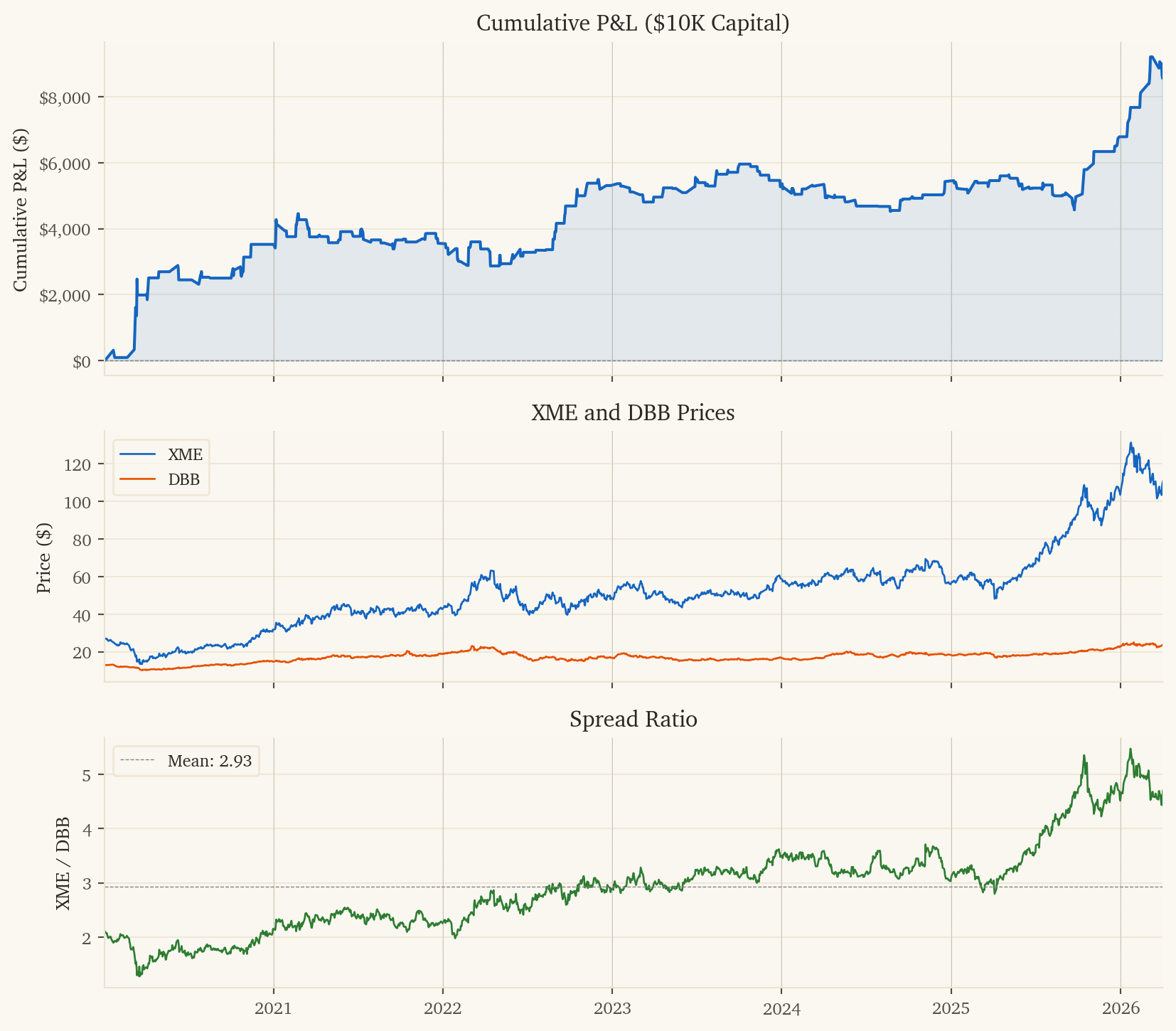
SELECT dt, spread AS spread_ret,
example.main.vgi_dynamic_ml_agg(
(SELECT code FROM agg_defs WHERE name = 'model'),
MAP {
'conf': 0.60, 'min_move': 0.001,
'corr_delta_max': 0.10, 'corr_delta_col': 4,
'svol_max': 0.40, 'svol_col': 5
},
spread, aud_ret, tlt_ret, dow_cos,
corr_delta, svol20_ann
) OVER (
ORDER BY t
ROWS BETWEEN 200 PRECEDING AND 1 PRECEDING
) AS prediction
FROM features
WHERE svol20_ann IS NOT NULL AND corr_delta IS NOT NULL;
-- 5. Trade: sign(prediction) = direction, binary sizing