How SQL Window Functions Train a ML Model
A single VGI aggregate powers all 8 strategies in this portfolio
What This Page Explains
Every strategy in this portfolio — from the daily commodity-momentum sleeves to the 10-day fixed-income mean-reversion sleeve — is implemented as one DuckDB SQL query using the same custom aggregate function: vgi_dynamic_ml_agg.
This function is defined in Python, executes inside a worker process via the VGI DuckDB extension, and runs as a window aggregate over historical rows. The window structure is what makes the backtest leak-free: the model only ever sees rows that occurred strictly before the row it’s predicting.
This page shows how the integration works, how the aggregate is defined in Python, and how the same infrastructure synthesises wildly different strategies just by changing input columns and parameters.
Architecture
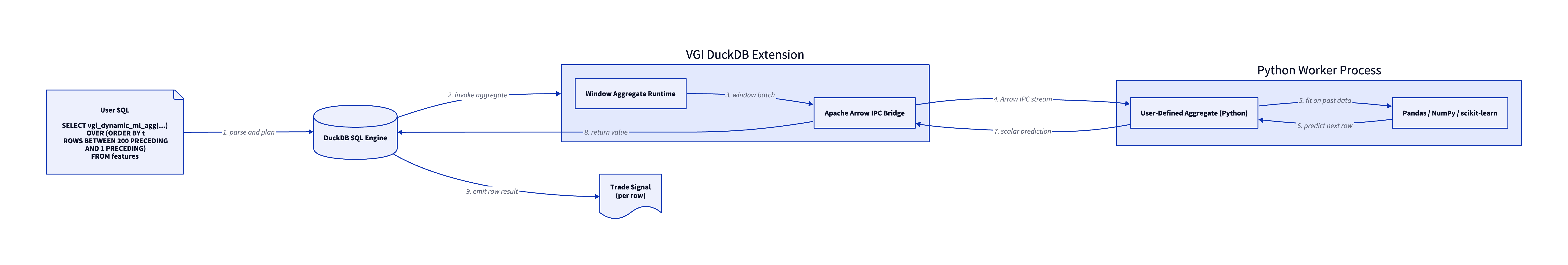
VGI is an in-progress DuckDB extension that bridges DuckDB’s columnar execution engine to a Python (or any language with an Apache Arrow implementation) worker process via Arrow IPC. The worker hosts user-defined aggregate functions; the extension handles serialization, windowing, and result return.
When DuckDB encounters vgi_dynamic_ml_agg(...) OVER (ORDER BY t ROWS BETWEEN 200 PRECEDING AND 1 PRECEDING):
- DuckDB plans the query and identifies the window aggregate
- For each output row, DuckDB streams the trailing 200 rows to the VGI extension
- VGI packages those rows as an Apache Arrow batch and ships them to the Python worker
- The Python aggregate function receives the batch as a
pyarrow.Table, fits a model on the past, predicts on the most recent row - The scalar prediction returns through VGI back to DuckDB
- DuckDB emits the prediction as the value for that row
The Window That Prevents Look-Ahead Bias
The single most important detail is the OVER clause:
example.main.vgi_dynamic_ml_agg(
  (SELECT code FROM agg_defs WHERE name='model'),
  MAP {'conf': 0.60, 'min_move': 0.008, 'fwd_col': 4, 'hold': 10},
  spread, pff_vs_hyg, ratio_zscore60, curve_mom120, spread_10d_fwd
) OVER (ORDER BY t ROWS BETWEEN 200 PRECEDING AND 1 PRECEDING) AS pred
ROWS BETWEEN 200 PRECEDING AND 1 PRECEDING is the leak-prevention guarantee. For row t, the aggregate sees rows t-200 through t-1. The current row’s outcome and all future rows are invisible. Even though the table contains forward-looking columns like spread_10d_fwd, the aggregate can only ever look at past values of those columns when fitting the model — and a past value of spread_10d_fwd is the realised return that was already known by the time the model trains.
This is conceptually equivalent to walk-forward cross-validation, but expressed as a single SQL aggregate that DuckDB handles natively.
The Aggregate in Python
The same Python aggregate is used (with minor parameter variations) across all 8 strategies. It’s defined as code stored in a DuckDB table at backtest time, then passed to the VGI worker as a string:
class Aggregate:
    @staticmethod
    def finalize(table, params):
        # `table` is the pyarrow.Table for the window:
        # rows = the trailing N rows (200 in our backtests)
        # columns = the feature columns + the forward-return target
        if table.num_rows < 2:
            return None

        data = table.to_pandas().values.astype(np.float64)
        n, nc = data.shape
        seed = int(params.get('seed', 42))
        conf_thresh = params.get('conf', 0.60)
        min_move = params.get('min_move', 0.008)
        fc = int(params.get('fwd_col', nc - 1))   # last column = target
        hold = int(params.get('hold', 10))         # holding period

        if n < 10 + hold:
            return None

        # Training set: features at time t paired with the realised
        # forward return that occurred at t+hold. The slicing gap
        # ensures no peeking.
        X = data[:-(hold), :fc]
        y_ret = data[hold:, fc]

        if np.any(np.isnan(X)) or np.any(np.isnan(y_ret)):
            return 0.0

        y_dir = (y_ret > 0).astype(int)
        last = data[-1:, :fc]   # the row we're predicting

        from sklearn.linear_model import LogisticRegression, Ridge
        from sklearn.pipeline import make_pipeline
        from sklearn.preprocessing import StandardScaler

        if len(set(y_dir)) < 2:
            return 0.0

        # Direction model
        clf = make_pipeline(
            StandardScaler(),
            LogisticRegression(C=0.1, max_iter=1000, random_state=seed)
        )
        clf.fit(X, y_dir)
        prob_up = clf.predict_proba(last)[0][1]

        # Magnitude model
        reg = make_pipeline(StandardScaler(), Ridge(alpha=1.0))
        reg.fit(X, y_ret)
        pred_mag = abs(float(reg.predict(last)[0]))

        if pred_mag < min_move:
            return 0.0
        if prob_up > conf_thresh:
            return pred_mag           # signed up
        elif prob_up < (1.0 - conf_thresh):
            return -pred_mag          # signed down
        else:
            return 0.0                # no trade
The function returns a single scalar per row: a signed predicted magnitude (positive = long the spread, negative = short, zero = no trade).
The Dual-Model Architecture (scikit-learn)
![]()
Each call to the aggregate function trains two scikit-learn models on the same trailing window of data, then combines their outputs into a single signal. This direction-plus-magnitude separation is one of the design choices that holds the whole portfolio together.
Why two models?
Predicting which way a spread will move and predicting how far it will move are different statistical problems. Mixing them into a single regression dilutes both signals — the regression’s loss is dominated by large outliers, while the directional signal has many close-to-zero observations that mislead a single model. Splitting them lets each algorithm do what it’s good at:
| Model | Library Class | Question It Answers | Why This Algorithm |
|---|---|---|---|
| Direction | LogisticRegression (C=0.1) |
Will the spread move up or down over the next N days? | L2-regularised logistic gives calibrated predict_proba outputs — we can demand prob_up > 0.60 (or < 0.40) before trading. |
| Magnitude | Ridge (alpha=1.0) |
If we trade, how big will the move be? | L2-regularised regression on the same features gives a magnitude estimate that survives the small-sample, many-feature regime (~190 rows × 4 features per fit). |
Both are wrapped in make_pipeline with StandardScaler so feature scales don’t dominate the regularisation. The same scaling is applied to the prediction row.
How they combine
clf = make_pipeline(StandardScaler(),
                    LogisticRegression(C=0.1, max_iter=1000, random_state=seed))
clf.fit(X, y_dir)
prob_up = clf.predict_proba(last)[0][1]

reg = make_pipeline(StandardScaler(), Ridge(alpha=1.0))
reg.fit(X, y_ret)
pred_mag = abs(float(reg.predict(last)[0]))

if pred_mag < min_move:           # Magnitude gate
    return 0.0
if prob_up > conf_thresh:         # Direction confidence (e.g. > 0.60)
    return  pred_mag
elif prob_up < (1.0 - conf_thresh):
    return -pred_mag
else:
    return 0.0                    # Neither side confident — flat
Two gates control trade entry:
- Magnitude gate (
pred_mag >= min_move): the predicted move must be large enough to clear transaction costs. Typical threshold0.005to0.008(50–80 bps over the holding period). - Direction gate (
|prob_up - 0.5| >= conf_thresh - 0.5): the classifier must be confident in the sign. We requireprob_up > 0.60for longs or< 0.40for shorts — anything in between is a no-trade.
The output is a single signed scalar per row — positive to go long the spread, negative to go short, zero to sit out. Both models retrain from scratch on every row, on the trailing 200 days. There is no global model state; the entire learning loop happens inside the window. This is exactly what walk-forward cross-validation does in conventional backtest harnesses, except here it’s free — it’s just the natural semantics of a SQL window aggregate.
What gets trained per row
For a 6-year backtest at one trade-day per row with a 200-day window, each strategy fits roughly 3,000 LogisticRegression models and 3,000 Ridge models — about 6,000 sklearn .fit() calls per backtest, all driven by a single SELECT statement. The Python worker does this in seconds because the models are tiny (4 features × ~190 samples), and the dominant cost is actually Arrow IPC overhead between DuckDB and Python — which VGI keeps minimal.
Easy Synthesis Across Strategies
The same aggregate function powers wildly different strategies because the semantics live in the input columns and parameters, not the function. A few examples:
XLF / XLY (Strategy 5) — 3-day sector rotation
example.main.vgi_dynamic_ml_agg(
  (SELECT code FROM agg_defs WHERE name='model'),
  MAP {'conf': 0.60, 'min_move': 0.008, 'fwd_col': 4, 'hold': 3},
  spread, corr_delta, gld_ret, kre_ret, spread_3d_fwd
) OVER (ORDER BY t ROWS BETWEEN 200 PRECEDING AND 1 PRECEDING) AS pred
Features: spread, correlation regime delta, gold return, regional bank return. Target: 3-day forward spread return. Hold for 3 days.
TLT / HYG (Strategy 7) — 10-day fixed-income mean reversion
example.main.vgi_dynamic_ml_agg(
  (SELECT code FROM agg_defs WHERE name='model'),
  MAP {'conf': 0.60, 'min_move': 0.008, 'fwd_col': 4, 'hold': 10},
  spread, pff_vs_hyg, ratio_zscore60, curve_mom120, spread_10d_fwd
) OVER (ORDER BY t ROWS BETWEEN 200 PRECEDING AND 1 PRECEDING) AS pred
Features: spread, credit positioning, 60d cumulative-ratio z-score, 120d yield-curve momentum. Target: 10-day forward spread return. Hold for 10 days.
LMT / RTX (Strategy 6) — 3-day defense sector pair
example.main.vgi_dynamic_ml_agg(
  (SELECT code FROM agg_defs WHERE name='model'),
  MAP {'conf': 0.60, 'min_move': 0.008, 'fwd_col': 4, 'hold': 3},
  spread, btc_mom20, month_sin, real_rate_ret, spread_3d_fwd
) OVER (ORDER BY t ROWS BETWEEN 200 PRECEDING AND 1 PRECEDING) AS pred
Features: spread, Bitcoin momentum, calendar seasonality, TIPS return. Target: 3-day forward spread return. Hold for 3 days.
The model code, the windowing, the leak-prevention — all identical. Only the columns being fed in and the holding period differ. This is what makes feature/strategy research fast: you can sweep across hundreds of feature combinations and holding periods using only SQL, with no special harness or data-pipeline plumbing.
Why This Matters for Research
Conventional backtest infrastructure couples features, models, and execution into bespoke Python pipelines. Each new strategy variant requires reimplementation. With VGI:
- One SQL query = one full backtest. No pipeline scaffolding.
- Walk-forward cross-validation is free. It’s the natural semantics of a window aggregate.
- The aggregate function is composable in any Python ML library — sklearn, XGBoost, PyTorch, statsmodels — because the worker is just Python.
- Parameter sweeps are SQL files. Change
'hold': 3to'hold': 10and rerun. Run 20 variants in parallel as 20 SQL files via DuckDB CLI. - The same DuckDB query that researches a strategy can be productionised — the aggregate is just a SQL UDF.
In this portfolio, this approach let us synthesise 8 production-quality strategies from a 179-feature library in a handful of compute-hours, with zero per-strategy framework code.
Learn More
VGI is an in-development DuckDB extension. If you’d like to use it for your own quant research, custom aggregates, or production data pipelines — or you want early access to the extension — please reach out: [email protected].
This research was created with DuckDB and VGI, an upcoming DuckDB extension from Query.Farm that allows custom aggregate functions to be written in any language with an Apache Arrow implementation.