Quant Strategy Research with Query.Farm’s VGI and DuckDB

Eight Uncorrelated Pairs Strategies

Eight uncorrelated pairs strategies driven from a single SQL window aggregate (https://duckdb.org/docs/stable/sql/functions/window_functions). On every row, the aggregate trains two scikit-learn models on the trailing 200 rows — ~50,000 fits per backtest, all driven by SQL.
Author
Affiliation

Rusty Conover

Query.Farm

Published

April 16, 2026

Show code
import sys, pandas as pd, numpy as np
import matplotlib.pyplot as plt
import matplotlib.dates as mdates
from matplotlib.patches import Patch
import warnings
warnings.filterwarnings('ignore')

sys.path.insert(0, '/Users/rusty/Development/trading')
from farm_theme import apply as apply_farm_theme, STRAT_COLORS, BENCH_COLORS, palette
apply_farm_theme()

capital = 10000

# Load all eight strategies
strategies = {
    'xme_dbb': '/Users/rusty/Development/trading/strategy1/docs/strategy_data.csv',
    'gdx_gld': '/Users/rusty/Development/trading/strategy2/docs/strategy_data.csv',
    'xle_uso': '/Users/rusty/Development/trading/strategy3/docs/strategy_data.csv',
    'efa_spy': '/Users/rusty/Development/trading/strategy4/docs/strategy_data.csv',
    'xlf_xly': '/Users/rusty/Development/trading/strategy5/docs/strategy_data.csv',
    'lmt_rtx': '/Users/rusty/Development/trading/strategy6/docs/strategy_data.csv',
    'tlt_hyg': '/Users/rusty/Development/trading/strategy7/docs/strategy_data.csv',
    'mtum_usmv': '/Users/rusty/Development/trading/strategy8/docs/strategy_data.csv',
}

dfs = {}
for name, path in strategies.items():
    df = pd.read_csv(path, parse_dates=['dt'])
    df.rename(columns={'daily_ret_unscaled': f'{name}_ret', 'active': f'{name}_active',
                        'pred': f'{name}_pred'}, inplace=True)
    dfs[name] = df[['dt', f'{name}_ret', f'{name}_active', f'{name}_pred']]

# Merge all on date
port = dfs['xme_dbb']
for name in ['gdx_gld', 'xle_uso', 'efa_spy', 'xlf_xly', 'lmt_rtx', 'tlt_hyg', 'mtum_usmv']:
    port = port.merge(dfs[name], on='dt', how='outer')

port = port.sort_values('dt').reset_index(drop=True)
port = port.fillna(0)

strat_names = list(strategies.keys())
strat_colors = STRAT_COLORS
strat_labels = {'xme_dbb': 'XME/DBB (metals)', 'gdx_gld': 'GDX/GLD (gold)',
                'xle_uso': 'XLE/USO (energy)', 'efa_spy': 'EFA/SPY (intl equity)',
                'xlf_xly': 'XLF/XLY (financials/discretionary)',
                'lmt_rtx': 'LMT/RTX (defense)',
                'tlt_hyg': 'TLT/HYG (rates/credit)',
                'mtum_usmv': 'MTUM/USMV (factor rotation)'}

# Allocation methods on total capital (10K per sleeve)
N_STRATS = len(strat_names)
total_capital = capital * N_STRATS  # $10K * N sleeves

port['n_active'] = sum(port[f'{s}_active'].astype(bool).astype(int) for s in strat_names)

# === Allocation A: Dedicated sleeves (1x) ===
# Each strategy gets fixed $10K. Idle when not active.
port['port_ret'] = sum(port[f'{s}_ret'] for s in strat_names) / N_STRATS

# === Allocation B: Concentrated active ===
# Total capital rotates onto active strategies, equal-weighted among them.
port['port_ret_concentrated'] = np.where(port['n_active'] > 0,
    sum(port[f'{s}_ret'] for s in strat_names) / port['n_active'],
    0.0)

# === Allocation C: Leveraged sleeves ===
# Each strategy gets $10K equity but trades at Lx notional.
# Pair trades (long X, short Y) are capital-efficient — broker margin offsets.
# Assume 50bps/yr financing cost per turn of leverage above 1x.
LEVERAGE_LEVELS = [1.5, 2.0, 3.0]
BORROW_RATE = 0.005  # 50 bps annual per turn of leverage
DAILY_BORROW = BORROW_RATE / 252

for L in LEVERAGE_LEVELS:
    # Daily borrow cost when any strategy is active (capital deployed)
    borrow_cost = (L - 1) * DAILY_BORROW * (port['n_active'] > 0).astype(float)
    port[f'port_lev{L}_ret'] = port['port_ret'] * L - borrow_cost

# Cumulative P&L (each strategy on its own $10K, for individual chart)
for s in strat_names:
    port[f'{s}_cum'] = (port[f'{s}_ret'] * capital).cumsum()

# Combined PnL on total equity
port['port_cum'] = (port['port_ret'] * total_capital).cumsum()
port['port_concentrated_cum'] = (port['port_ret_concentrated'] * total_capital).cumsum()
for L in LEVERAGE_LEVELS:
    port[f'port_lev{L}_cum'] = (port[f'port_lev{L}_ret'] * total_capital).cumsum()
port['port_dd'] = port['port_cum'] - port['port_cum'].cummax()
port['year'] = port['dt'].dt.year

# Load benchmarks (SPY, QQQ, IWM buy and hold)
benchmarks = {}
for ticker, label, color in [('SPY', 'SPY (buy & hold)', '#9E9E9E'),
                              ('QQQ', 'QQQ (buy & hold)', '#5E35B1'),
                              ('IWM', 'IWM (buy & hold)', '#00897B')]:
    bdf = pd.read_csv(f'/Users/rusty/Development/trading/explore_intl/data/{ticker}.csv', parse_dates=['Date'])
    bdf = bdf[bdf['Date'] >= port['dt'].min()].sort_values('Date').reset_index(drop=True)
    # Compute cumulative P&L on total_capital invested at start
    first_close = bdf['close'].iloc[0]
    bdf[f'{ticker}_cum'] = (bdf['close'] / first_close - 1) * total_capital
    benchmarks[ticker] = (bdf[['Date', f'{ticker}_cum']].rename(columns={'Date': 'dt'}), label, color)
TipWhat This Is

DuckDB scikit-learn

This portfolio is a demonstration of VGI — an upcoming DuckDB extension from Query.Farm that lets you host custom aggregate functions written in any language with an Apache Arrow implementation.

This is a complete, end-to-end ML-enabled trading portfolio expressed entirely in SQL — feature engineering, feature selection, model training, walk-forward cross-validation, and backtest accounting are all SQL queries against DuckDB. There is no separate Python harness driving the experiment loop; SQL is the experiment loop.

Every strategy here is generated by a single SQL window aggregate (vgi_dynamic_ml_agg) that, on each row, trains two scikit-learn models from scratch — a LogisticRegression for direction and a Ridge for magnitude — on the trailing 200 rows. The aggregate’s Python source is stored as a string inside DuckDB itself (in an agg_defs table) and executed by the VGI worker on demand — no recompilation, no separate ML pipeline, no walk-forward harness. The leak-prevention is just the natural semantics of a SQL window function: ROWS BETWEEN 200 PRECEDING AND 1 PRECEDING.

Keeping the whole stack in SQL has two compounding benefits:

  • DuckDB’s vectorised execution does the heavy lifting — feature scans across 179 candidate features and 13 candidate pairs run in parallel across all cores with no manual orchestration.
  • Coding agents extend it trivially. Adding a new strategy is “write a SQL file”; adding a new feature is “append to a YAML”; adding a new pair is “run one Python script that emits SQL.” The shape of the work is uniform, which means an LLM can generate, test, and iterate on strategies with very little scaffolding.

This makes high-throughput strategy research practical: 8 strategies × ~6,000 model fits each = roughly 50,000 model trainings driven entirely from SQL.

 Learn how VGI extends DuckDB aggregate functions →

WarningNot Investment Advice

This is research output, not a recommendation to trade. All results are in-sample backtests selected through extensive parameter and pair search — they reflect the period 2020–2026 and one full Fed cycle. Any real-world deployment needs substantial out-of-sample paper-trading (3–6 months minimum) before risking capital, and you should expect post-deployment Sharpe ratios materially below the backtest figures. Past performance does not predict future returns. Trade at your own risk.

The Portfolio at a Glance

This portfolio runs eight independent pairs trading strategies across commodities, precious metals, energy, geographic equity rotation, US sector rotation, US defense sector, fixed-income (rates vs credit), and US equity factor rotation. Each strategy predicts spread divergences between two related ETFs or stocks using a different set of macro signals. The strategies are nearly uncorrelated with each other and with major asset classes — the defense (LMT/RTX) and rates/credit (TLT/HYG) sleeves actively hedge drawdowns in the equity and commodity sleeves.

Show code
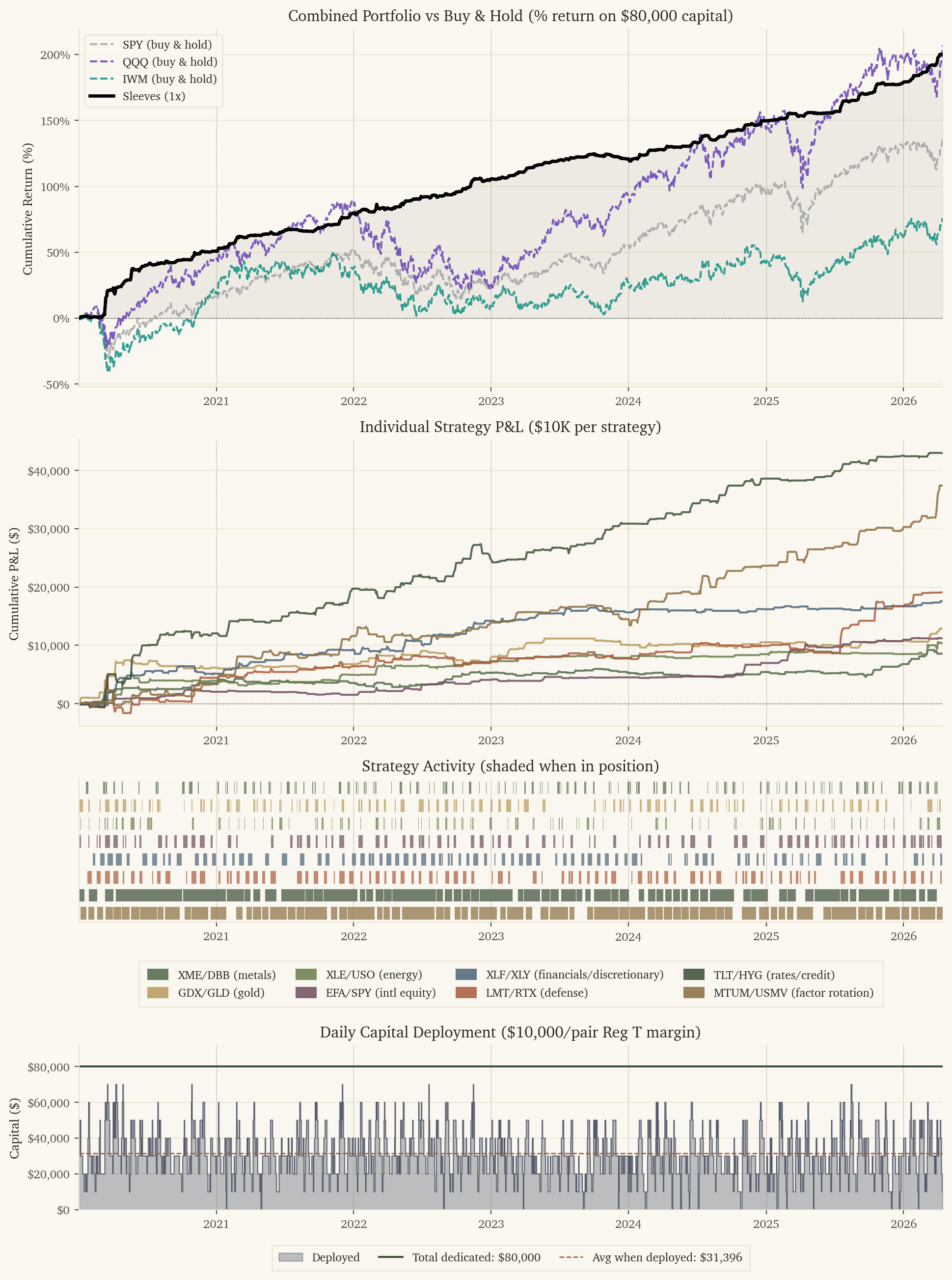
# Capital per pair trade: $10K long + $10K short = $10K margin (Reg T 50%)
MARGIN_PER_PAIR = 10000

from matplotlib.gridspec import GridSpec
fig = plt.figure(figsize=(10, 13.5), constrained_layout=True)
gs = GridSpec(5, 1, height_ratios=[2.5, 2, 1, 0.4, 1.15], figure=fig)
ax1 = fig.add_subplot(gs[0])
ax_strat = fig.add_subplot(gs[1], sharex=ax1)
ax2 = fig.add_subplot(gs[2], sharex=ax1)
ax_legend = fig.add_subplot(gs[3])
ax_legend.axis('off')  # spacer row reserved for the strategy legend
ax3 = fig.add_subplot(gs[4], sharex=ax1)

# Panel 1: Combined Portfolio (two allocation methods) vs benchmarks — in percent
for ticker, (bdf, label, color) in benchmarks.items():
    ax1.plot(bdf['dt'], bdf[f'{ticker}_cum'] / total_capital * 100,
             color=color, linewidth=1.5, linestyle='--', alpha=0.8, label=label, zorder=3)

ax1.plot(port['dt'], port['port_cum'] / total_capital * 100,
         color='black', linewidth=2.5, label='Sleeves (1x)', zorder=5)
ax1.fill_between(port['dt'], 0, port['port_cum'] / total_capital * 100, alpha=0.05, color='black')
ax1.axhline(y=0, color='gray', linewidth=0.5, linestyle='--')

for yr in range(port['dt'].dt.year.min(), port['dt'].dt.year.max() + 2):
    for ax in [ax1, ax_strat, ax2, ax3]:
        ax.axvline(x=pd.Timestamp(f'{yr}-01-01'), color='gray', linewidth=0.3, linestyle=':')

ax1.set_ylabel('Cumulative Return (%)')
ax1.set_title(f'Combined Portfolio vs Buy & Hold (% return on ${total_capital:,} capital)')
ax1.yaxis.set_major_formatter(plt.FuncFormatter(lambda x, _: f'{x:.0f}%'))
ax1.legend(loc='upper left', fontsize=9)

# Panel 2: Individual strategies (own scale) — colors shared with activity below
for s in strat_names:
    ax_strat.plot(port['dt'], port[f'{s}_cum'], color=strat_colors[s], linewidth=1.5,
                  alpha=0.85, label=strat_labels[s])
ax_strat.axhline(y=0, color='gray', linewidth=0.5, linestyle='--')
ax_strat.set_ylabel('Cumulative P&L ($)')
ax_strat.set_title('Individual Strategy P&L ($10K per strategy)')
ax_strat.yaxis.set_major_formatter(plt.FuncFormatter(lambda x, _: f'${x:,.0f}'))

# Panel 2: Strategy activity — one horizontal lane per strategy, shaded when active
# Active = pred != 0 OR holding open position
hold_periods = {'xme_dbb': 1, 'gdx_gld': 2, 'xle_uso': 1, 'efa_spy': 3, 'xlf_xly': 3,
                'lmt_rtx': 3, 'tlt_hyg': 10, 'mtum_usmv': 10}

# For each strategy, compute "in position" days (active OR holding from prior entry)
for s in strat_names:
    hold = hold_periods[s]
    active = port[f'{s}_active'].astype(bool).values
    # Forward-fill: a position entered on day i is held for `hold` days
    in_position = np.zeros(len(active), dtype=bool)
    for i in range(len(active)):
        if active[i]:
            for j in range(hold):
                if i + j < len(active):
                    in_position[i + j] = True
    port[f'{s}_in_position'] = in_position

# Plot one horizontal lane per strategy
lane_height = 0.7
for idx, s in enumerate(strat_names):
    y_pos = len(strat_names) - 1 - idx  # top-to-bottom order
    in_pos = port[f'{s}_in_position'].values
    # Find contiguous runs of activity for cleaner rendering
    in_run = False
    run_start = None
    for i, active in enumerate(in_pos):
        if active and not in_run:
            run_start = port['dt'].iloc[i]
            in_run = True
        elif not active and in_run:
            run_end = port['dt'].iloc[i]
            ax2.barh(y_pos, run_end - run_start, left=run_start,
                    height=lane_height, color=strat_colors[s], alpha=0.7)
            in_run = False
    if in_run:
        run_end = port['dt'].iloc[-1] + pd.Timedelta(days=1)
        ax2.barh(y_pos, run_end - run_start, left=run_start,
                height=lane_height, color=strat_colors[s], alpha=0.7)

ax2.set_yticks([])
ax2.set_title('Strategy Activity (shaded when in position)')
ax2.set_ylim(-0.5, len(strat_names) - 0.5)
ax2.grid(axis='y', visible=False)
ax2.set_ylabel('')

# Shared legend on its dedicated spacer axis — color swatches for each strategy
legend_handles = [Patch(facecolor=strat_colors[s], alpha=0.85, label=strat_labels[s])
                  for s in strat_names]
ax_legend.legend(handles=legend_handles, loc='center', ncol=4, frameon=True,
                 fancybox=False, fontsize=9, columnspacing=1.6, handlelength=1.8,
                 handleheight=1.1, borderpad=0.7)

# Panel 3: Capital deployed per day
# Each strategy has $10K dedicated capital sitting in account at all times.
# When active (in position), capital is deployed; otherwise it's idle cash.
port['n_in_position'] = sum(port[f'{s}_in_position'].astype(int) for s in strat_names)
port['capital_deployed'] = port['n_in_position'] * MARGIN_PER_PAIR

ax3.fill_between(port['dt'], port['capital_deployed'], 0, color=palette('slate'), alpha=0.35, step='mid', label='Deployed')
ax3.plot(port['dt'], port['capital_deployed'], color=palette('slate'), linewidth=0.5, drawstyle='steps-mid')

# Show total dedicated capital line
ax3.axhline(y=total_capital, color=palette('sage-dark'), linewidth=1.5, linestyle='-',
            label=f'Total dedicated: ${total_capital:,}')

avg_deployed = port.loc[port['capital_deployed'] > 0, 'capital_deployed'].mean()
ax3.axhline(y=avg_deployed, color=palette('rust'), linewidth=1, linestyle='--',
            label=f'Avg when deployed: ${avg_deployed:,.0f}')

ax3.set_ylabel('Capital ($)')
ax3.set_title(f'Daily Capital Deployment (${MARGIN_PER_PAIR:,}/pair Reg T margin)')
ax3.yaxis.set_major_formatter(plt.FuncFormatter(lambda x, _: f'${x:,.0f}'))
ax3.set_ylim(0, total_capital * 1.15)
ax3.set_xlim(port['dt'].min(), port['dt'].max())
ax3.legend(loc='upper center', bbox_to_anchor=(0.5, -0.18), ncol=3,
           frameon=True, fancybox=False, fontsize=9, columnspacing=1.6,
           handlelength=2.0, borderpad=0.6)

# Constrained layout (above) auto-fits titles/legends/labels — no manual margins needed.
# Add a touch of breathing room around the entire figure.
fig.get_layout_engine().set(w_pad=0.05, h_pad=0.06, hspace=0.05, wspace=0.05)
plt.savefig('portfolio_overview.png', dpi=110, bbox_inches='tight', facecolor='white')
plt.show()
Figure 1: Portfolio cumulative P&L and individual strategy contributions
Show code
# Compute stats for each strategy and the combined portfolio from the data
def strat_stats(rets, name):
    traded = rets[rets != 0]
    if len(traded) < 2:
        return {}
    sharpe = traded.mean() / traded.std() * np.sqrt(252)
    pnl = (rets * capital).sum()
    acc_col = f'{name}_pred' if f'{name}_pred' in port.columns else None
    if acc_col:
        active_mask = port[f'{name}_active'].astype(bool)
        correct = (np.sign(port.loc[active_mask, acc_col]) == np.sign(port.loc[active_mask, f'{name}_ret'])).mean() * 100
    else:
        correct = np.nan
    # After 10bps
    net = traded - 0.001
    net_sharpe = net.mean() / net.std() * np.sqrt(252) if len(net) > 1 else 0
    # Years positive
    yr_pnl = port.groupby('year').apply(lambda g: (g[f'{name}_ret'] * capital).sum())
    yrs_pos = f'{(yr_pnl > 0).sum()}/{len(yr_pnl)}'
    return {
        'Sharpe': f'{sharpe:.2f}',
        'PnL': f'${pnl:,.0f}',
        'Accuracy': f'{correct:.1f}%' if not np.isnan(correct) else '--',
        'Years +': yrs_pos,
        'Post-10bps': f'{net_sharpe:.2f}',
    }

hold_map = {'xme_dbb': 'Daily', 'gdx_gld': '2-day', 'xle_uso': 'Daily',
            'efa_spy': '3-day', 'xlf_xly': '3-day', 'lmt_rtx': '3-day',
            'tlt_hyg': '10-day', 'mtum_usmv': '10-day'}
signal_map = {'xme_dbb': 'AUD, corr delta', 'gdx_gld': 'CHF+JPY, gold-silver',
              'xle_uso': 'TLT, credit, curve', 'efa_spy': 'safe haven, oil, AUD',
              'xlf_xly': 'corr delta, gold, KRE',
              'lmt_rtx': 'BTC mom, season, real rates',
              'tlt_hyg': 'PFF-HYG, ratio z, curve cycle',
              'mtum_usmv': 'KRE-XLF, gold, financials'}

rows = {}
for s in strat_names:
    traded_rets = port.loc[port[f'{s}_active'].astype(bool), f'{s}_ret']
    st = strat_stats(traded_rets, s)
    st['Hold'] = hold_map[s]
    st['Key signal'] = signal_map[s]
    rows[strat_labels[s]] = st

# Combined stats — PnL computed on total capital, equals sum of individuals
port_traded = port.loc[port['port_ret'] != 0, 'port_ret']
port_sharpe = port_traded.mean() / port_traded.std() * np.sqrt(252)
port_pnl = (port['port_ret'] * total_capital).sum()
# Net Sharpe with 10bps cost on each active strategy
port_net_rets = port.apply(lambda r: (
    sum(r[f'{s}_ret'] - 0.001 if r[f'{s}_active'] else 0 for s in strat_names) / N_STRATS
), axis=1)
port_net_traded = port_net_rets[port_net_rets != 0]
port_net_sharpe = port_net_traded.mean() / port_net_traded.std() * np.sqrt(252)
yr_pnl_comb = port.groupby('year').apply(lambda g: (g['port_ret'] * total_capital).sum())
rows['**Combined**'] = {
    'Sharpe': f'**{port_sharpe:.2f}**',
    'PnL': f'**${port_pnl:,.0f}**',
    'Accuracy': '--',
    'Years +': f'**{(yr_pnl_comb > 0).sum()}/{len(yr_pnl_comb)}**',
    'Hold': '--',
    'Key signal': '--',
    'Post-10bps': f'**{port_net_sharpe:.2f}**',
}

summary_df = pd.DataFrame(rows).T
summary_df.index.name = 'Strategy'
display(summary_df)
Table 1
Sharpe PnL Accuracy Years + Post-10bps Hold Key signal
Strategy
XME/DBB (metals) 2.56 $8,577 51.2% 6/7 1.79 Daily AUD, corr delta
GDX/GLD (gold) 2.92 $12,888 47.4% 7/7 2.36 2-day CHF+JPY, gold-silver
XLE/USO (energy) 3.04 $10,395 50.6% 7/7 2.52 Daily TLT, credit, curve
EFA/SPY (intl equity) 5.30 $11,214 48.6% 6/7 4.14 3-day safe haven, oil, AUD
XLF/XLY (financials/discretionary) 4.65 $17,572 51.5% 7/7 3.93 3-day corr delta, gold, KRE
LMT/RTX (defense) 2.65 $19,080 49.8% 7/7 2.26 3-day BTC mom, season, real rates
TLT/HYG (rates/credit) 6.49 $42,987 43.3% 7/7 5.86 10-day PFF-HYG, ratio z, curve cycle
MTUM/USMV (factor rotation) 5.63 $37,398 52.5% 7/7 5.08 10-day KRE-XLF, gold, financials
**Combined** **5.61** **$160,110** -- **7/7** **4.86** -- --

How the Strategies Complement Each Other

Show code
years = sorted(port['year'].unique())
yearly = port.groupby('year').agg(
    xme=('xme_dbb_ret', lambda x: (x * capital).sum()),
    gdx=('gdx_gld_ret', lambda x: (x * capital).sum()),
    xle=('xle_uso_ret', lambda x: (x * capital).sum()),
    efa=('efa_spy_ret', lambda x: (x * capital).sum()),
    xlf=('xlf_xly_ret', lambda x: (x * capital).sum()),
    lmt=('lmt_rtx_ret', lambda x: (x * capital).sum()),
    tlt=('tlt_hyg_ret', lambda x: (x * capital).sum()),
    mtum=('mtum_usmv_ret', lambda x: (x * capital).sum()),
    combined=('port_ret', lambda x: (x * total_capital).sum()),
).reset_index()

fig, ax = plt.subplots(figsize=(10, 5))

x = np.arange(len(years))
w = 0.10
ax.bar(x - 4*w, yearly['xme'], w, color='#1565C0', alpha=0.7, label='XME/DBB')
ax.bar(x - 3*w, yearly['gdx'], w, color='#FFB300', alpha=0.7, label='GDX/GLD')
ax.bar(x - 2*w, yearly['xle'], w, color='#2E7D32', alpha=0.7, label='XLE/USO')
ax.bar(x - 1*w, yearly['efa'], w, color='#7B1FA2', alpha=0.7, label='EFA/SPY')
ax.bar(x + 0*w, yearly['xlf'], w, color='#00838F', alpha=0.7, label='XLF/XLY')
ax.bar(x + 1*w, yearly['lmt'], w, color='#5D4037', alpha=0.7, label='LMT/RTX')
ax.bar(x + 2*w, yearly['tlt'], w, color='#D32F2F', alpha=0.7, label='TLT/HYG')
ax.bar(x + 3*w, yearly['mtum'], w, color='#6A1B9A', alpha=0.7, label='MTUM/USMV')
ax.bar(x + 4*w, yearly['combined'], w, color='black', alpha=0.8, label='Combined')

ax.set_xticks(x)
ax.set_xticklabels(years)
ax.axhline(y=0, color='gray', linewidth=0.5)
ax.set_ylabel('P&L ($)')
ax.set_title('Yearly P&L by Strategy')
ax.yaxis.set_major_formatter(plt.FuncFormatter(lambda x, _: f'${x:,.0f}'))
ax.legend(loc='upper left', fontsize=9)

plt.tight_layout()
plt.show()
Figure 2: Yearly P&L by strategy — when one is weak, others carry the portfolio
Show code
yearly_data = []
for yr in years:
    ydf = port[port['year'] == yr]
    pnls = {
        'XME/DBB': (ydf['xme_dbb_ret'] * capital).sum(),
        'GDX/GLD': (ydf['gdx_gld_ret'] * capital).sum(),
        'XLE/USO': (ydf['xle_uso_ret'] * capital).sum(),
        'EFA/SPY': (ydf['efa_spy_ret'] * capital).sum(),
        'XLF/XLY': (ydf['xlf_xly_ret'] * capital).sum(),
        'LMT/RTX': (ydf['lmt_rtx_ret'] * capital).sum(),
        'TLT/HYG': (ydf['tlt_hyg_ret'] * capital).sum(),
        'MTUM/USMV': (ydf['mtum_usmv_ret'] * capital).sum(),
    }
    comb_pnl = (ydf['port_ret'] * total_capital).sum()

    row = {'Year': yr}
    for name, pnl in pnls.items():
        row[name] = f'${pnl:,.0f}'
    row['Combined'] = f'${comb_pnl:,.0f}'
    row['Best'] = max(pnls, key=pnls.get)
    yearly_data.append(row)

pd.DataFrame(yearly_data).style.hide(axis='index')
Table 2: Yearly breakdown — note how strategies cover each other’s weak spots
Year XME/DBB GDX/GLD XLE/USO EFA/SPY XLF/XLY LMT/RTX TLT/HYG MTUM/USMV Combined Best
2020 $3,523 $6,190 $3,934 $2,046 $5,145 $4,444 $12,054 $3,332 $40,668 TLT/HYG
2021 $33 $584 $1,020 $-508 $4,007 $1,964 $7,667 $8,270 $23,037 MTUM/USMV
2022 $1,753 $930 $2,351 $2,550 $5,067 $547 $5,137 $2,300 $20,635 TLT/HYG
2023 $-39 $2,400 $566 $431 $1,434 $784 $6,003 $579 $12,159 TLT/HYG
2024 $160 $422 $622 $2,463 $542 $2,185 $7,719 $9,170 $23,284 MTUM/USMV
2025 $1,359 $213 $19 $3,988 $488 $6,819 $3,919 $6,507 $23,313 LMT/RTX
2026 $1,788 $2,148 $1,882 $243 $889 $2,337 $488 $7,240 $17,015 MTUM/USMV

Diversification Benefit

Show code
# Compute correlation on active-only returns
active_rets = port[['xme_dbb_ret', 'gdx_gld_ret', 'xle_uso_ret', 'efa_spy_ret', 'xlf_xly_ret', 'lmt_rtx_ret', 'tlt_hyg_ret', 'mtum_usmv_ret']].copy()
active_rets.columns = ['XME/DBB', 'GDX/GLD', 'XLE/USO', 'EFA/SPY', 'XLF/XLY', 'LMT/RTX', 'TLT/HYG', 'MTUM/USMV']

corr = active_rets.corr()
n = len(corr)

fig, ax = plt.subplots(figsize=(7, 6), constrained_layout=True)
im = ax.imshow(corr.values, cmap='RdBu_r', vmin=-1, vmax=1)
ax.set_xticks(range(n))
ax.set_xticklabels(corr.columns, fontsize=9, rotation=45, ha='right', rotation_mode='anchor')
ax.set_yticks(range(n))
ax.set_yticklabels(corr.index, fontsize=9)

for i in range(n):
    for j in range(n):
        color = 'white' if abs(corr.values[i, j]) > 0.5 else 'black'
        ax.text(j, i, f'{corr.values[i, j]:.2f}', ha='center', va='center', fontsize=10, color=color)

plt.colorbar(im, ax=ax, shrink=0.8)
ax.set_title('Return Correlation Matrix')
plt.show()
Figure 3: Return correlation matrix — the three strategies are nearly uncorrelated
Show code
# Count days by number of strategies in position (includes held positions, not just signals)
overlap_counts = port['n_in_position'].value_counts().sort_index()
total_days = len(port)

labels = ['No strategies\n(idle)', '1 strategy\nin position', '2 strategies\nin position',
          '3 strategies\nin position', '4 strategies\nin position', '5 strategies\nin position',
          '6 strategies\nin position', '7 strategies\nin position', '8 strategies\nin position']
colors = ['#BDBDBD', '#81C784', '#FFB74D', '#E57373', '#CE93D8', '#80DEEA', '#A1887F', '#EF9A9A', '#9FA8DA']

existing = [overlap_counts.get(i, 0) for i in range(9)]
pcts = [100 * v / total_days for v in existing]

fig, ax = plt.subplots(figsize=(10, 4))
bars = ax.bar(range(9), existing, color=colors, alpha=0.8, edgecolor='white')
ax.set_xticks(range(9))
ax.set_xticklabels(labels, fontsize=9)
ax.set_ylabel('Days')
ax.set_title(f'Capital Utilization Distribution ({total_days} total days)')
ax.yaxis.set_major_formatter(plt.FuncFormatter(lambda x, _: f'{int(x):,}'))

for bar, count, pct in zip(bars, existing, pcts):
    if count > 0:
        ax.text(bar.get_x() + bar.get_width()/2, bar.get_height() + total_days * 0.01,
                f'{count}\n({pct:.0f}%)', ha='center', va='bottom', fontsize=9)

ax.set_ylim(0, max(existing) * 1.15)
plt.tight_layout()
plt.show()
Figure 4: Capital utilization — how often each number of strategies is in position simultaneously (counting multi-day holds)

Risk Management

Show code
n = len(strat_names)
fig, axes = plt.subplots(n + 1, 1, figsize=(10, 1.6 * (n + 1)), sharex=True)

# Top panel: combined portfolio drawdown
ax0 = axes[0]
ax0.fill_between(port['dt'], port['port_dd'], 0, color='black', alpha=0.3)
ax0.plot(port['dt'], port['port_dd'], color='black', linewidth=1.2)
ax0.set_title(f'Combined Portfolio (${total_capital:,}) — Max: ${port["port_dd"].min():,.0f}', fontsize=11, loc='left', fontweight='bold')
ax0.yaxis.set_major_formatter(plt.FuncFormatter(lambda x, _: f'${x:,.0f}'))
ax0.tick_params(axis='both', labelsize=8)
for yr in range(port['dt'].dt.year.min(), port['dt'].dt.year.max() + 2):
    ax0.axvline(x=pd.Timestamp(f'{yr}-01-01'), color='gray', linewidth=0.3, linestyle=':')

# Per-strategy panels
for i, s in enumerate(strat_names):
    ax = axes[i + 1]
    dd = port[f'{s}_cum'] - port[f'{s}_cum'].cummax()
    ax.fill_between(port['dt'], dd, 0, color=strat_colors[s], alpha=0.4)
    ax.plot(port['dt'], dd, color=strat_colors[s], linewidth=0.8)
    ax.set_title(f'{strat_labels[s]} — Max: ${dd.min():,.0f}', fontsize=10, loc='left')
    ax.yaxis.set_major_formatter(plt.FuncFormatter(lambda x, _: f'${x:,.0f}'))
    ax.tick_params(axis='both', labelsize=8)
    for yr in range(port['dt'].dt.year.min(), port['dt'].dt.year.max() + 2):
        ax.axvline(x=pd.Timestamp(f'{yr}-01-01'), color='gray', linewidth=0.3, linestyle=':')

axes[-1].set_xlim(port['dt'].min(), port['dt'].max())
plt.tight_layout()
plt.show()
Figure 5: Combined portfolio drawdown (top) and per-strategy drawdowns, shared time axis

The Hidden Risk: Drawdown Correlation

Daily return correlations are low (the strategies look diversified day-to-day), but drawdown correlations are much higher because drawdowns persist for weeks or months. When you most need diversification — during stress — the strategies often lose together.

Show code
# Compute drawdowns for each strategy
dd_data = {}
for s in strat_names:
    cum = port[f'{s}_cum']
    dd_data[s] = (cum - cum.cummax()).values

dd_df = pd.DataFrame(dd_data)
dd_df.columns = [strat_labels[s].split(' (')[0] for s in strat_names]

ret_data = {strat_labels[s].split(' (')[0]: port[f'{s}_ret'].values for s in strat_names}
ret_df = pd.DataFrame(ret_data)

ret_corr = ret_df.corr()
dd_corr = dd_df.corr()

fig, (ax1, ax2) = plt.subplots(1, 2, figsize=(10, 4))

n = len(ret_corr)
for ax, corr, title in [(ax1, ret_corr, 'Daily Return Correlation'),
                         (ax2, dd_corr, 'Drawdown Correlation')]:
    im = ax.imshow(corr.values, cmap='RdBu_r', vmin=-1, vmax=1)
    ax.set_xticks(range(n))
    ax.set_xticklabels(corr.columns, fontsize=9, rotation=20, ha='right')
    ax.set_yticks(range(n))
    ax.set_yticklabels(corr.index, fontsize=9)
    for i in range(n):
        for j in range(n):
            color = 'white' if abs(corr.values[i, j]) > 0.5 else 'black'
            ax.text(j, i, f'{corr.values[i, j]:.2f}', ha='center', va='center',
                    fontsize=10, color=color)
    ax.set_title(title)

plt.tight_layout()
plt.show()
Figure 6: Daily return correlation vs drawdown correlation — drawdowns are 4x more correlated
Show code
# How many strategies are in DD on each day
in_dd = pd.DataFrame({s: (dd_data[s] < 0).astype(int) for s in strat_names})
n_in_dd = in_dd.sum(axis=1)

fig, (ax1, ax2) = plt.subplots(1, 2, figsize=(10, 4))

# Bar chart: days by # of strategies in DD
counts = n_in_dd.value_counts().sort_index()
total_days = len(n_in_dd)
labels = ['0\n(none)', '1', '2', '3', '4\n(all)']
colors = ['#43A047', '#81C784', '#FFB74D', '#E57373', '#B71C1C']
existing = [counts.get(i, 0) for i in range(5)]
pcts = [100 * v / total_days for v in existing]
bars = ax1.bar(range(5), existing, color=colors, alpha=0.8, edgecolor='white')
ax1.set_xticks(range(5))
ax1.set_xticklabels(labels, fontsize=10)
ax1.set_ylabel('Days')
ax1.set_title(f'Strategies Simultaneously In Drawdown ({total_days} days)')
for bar, count, pct in zip(bars, existing, pcts):
    if count > 0:
        ax1.text(bar.get_x() + bar.get_width()/2, bar.get_height() + total_days * 0.01,
                f'{count}\n({pct:.0f}%)', ha='center', va='bottom', fontsize=9)
ax1.set_ylim(0, max(existing) * 1.18)

# Stat per strategy: % of time in drawdown
strat_in_dd_pct = [100 * (dd_data[s] < 0).sum() / len(dd_data[s]) for s in strat_names]
strat_short_labels = [strat_labels[s].split(' (')[0] for s in strat_names]
bars2 = ax2.bar(range(len(strat_names)), strat_in_dd_pct,
                color=[strat_colors[s] for s in strat_names], alpha=0.8)
ax2.set_xticks(range(len(strat_names)))
ax2.set_xticklabels(strat_short_labels, fontsize=10, rotation=20, ha='right')
ax2.set_ylabel('% of Days in Drawdown')
ax2.set_title('Each Strategy: Time in Drawdown')
ax2.set_ylim(0, 105)
for bar, pct in zip(bars2, strat_in_dd_pct):
    ax2.text(bar.get_x() + bar.get_width()/2, bar.get_height() + 1.5,
            f'{pct:.0f}%', ha='center', va='bottom', fontsize=10)

plt.tight_layout()
plt.show()
Figure 7: Days simultaneously in drawdown — when one strategy is losing, others usually are too
Show code
avg_ret_corr = ret_corr.where(np.triu(np.ones(ret_corr.shape), k=1).astype(bool)).stack().mean()
avg_dd_corr = dd_corr.where(np.triu(np.ones(dd_corr.shape), k=1).astype(bool)).stack().mean()
all_in_dd = (n_in_dd == len(strat_names)).sum()
three_plus_in_dd = (n_in_dd >= 3).sum()

dd_summary = {
    'Avg pairwise daily-return correlation': f'{avg_ret_corr:.3f}',
    'Avg pairwise drawdown correlation': f'{avg_dd_corr:.3f}',
    'Drawdown correlation amplification': f'{avg_dd_corr / avg_ret_corr:.1f}x' if avg_ret_corr > 0 else 'N/A',
    'Days with all 8 strategies in drawdown': f'{all_in_dd} ({100*all_in_dd/total_days:.0f}%)',
    'Days with 3+ strategies in drawdown': f'{three_plus_in_dd} ({100*three_plus_in_dd/total_days:.0f}%)',
}
pd.DataFrame(list(dd_summary.items()), columns=['Metric', 'Value']).style.hide(axis='index')
Table 3
Metric Value
Avg pairwise daily-return correlation 0.016
Avg pairwise drawdown correlation 0.036
Drawdown correlation amplification 2.3x
Days with all 8 strategies in drawdown 206 (13%)
Days with 3+ strategies in drawdown 1547 (99%)
WarningWhy Drawdown Correlation Matters

Daily return correlation measures short-term dependency. Drawdown correlation measures path-dependent dependency. The latter is what determines actual portfolio drawdowns.

Even though daily returns are nearly uncorrelated, the strategies tend to be in drawdown at the same time because:

  1. Drawdowns persist — a single bad week can keep a strategy underwater for months
  2. Macro regime shifts affect multiple strategies simultaneously (rate hikes, COVID, geopolitical events)
  3. Volatility clustering — when one strategy starts losing, market conditions often cause others to lose too

This means the leveraged sleeves and concentrated allocations carry more tail risk than daily correlations suggest. Sizing for the average drawdown is dangerous; size for the joint drawdown.

Portfolio Statistics

Show code
traded_port = port[port['port_ret'] != 0]
sharpe_port = traded_port['port_ret'].mean() / traded_port['port_ret'].std() * np.sqrt(252)
downside_port = traded_port.loc[traded_port['port_ret'] < 0, 'port_ret']
sortino_port = traded_port['port_ret'].mean() / np.sqrt((downside_port**2).mean()) * np.sqrt(252)
max_dd_port = port['port_dd'].min()
ann_ret = traded_port['port_ret'].mean() * 252
total_pnl = (port['port_ret'] * total_capital).sum()
years_val = (port['dt'].max() - port['dt'].min()).days / 365.25
cagr = ((total_capital + total_pnl) / total_capital) ** (1/years_val) - 1

# After 10bps costs (cost applied to each active strategy)
net_rets = port.apply(lambda r: (
    sum(r[f'{s}_ret'] - 0.001 if r[f'{s}_active'] else 0 for s in strat_names) / N_STRATS
), axis=1)
net_traded = net_rets[net_rets != 0]
net_sharpe = net_traded.mean() / net_traded.std() * np.sqrt(252)

total_pnl_net = (net_rets * total_capital).sum()
cagr_net = ((total_capital + total_pnl_net) / total_capital) ** (1/years_val) - 1

# Concentrated allocation stats
conc_traded = port[port['port_ret_concentrated'] != 0]
conc_sharpe = conc_traded['port_ret_concentrated'].mean() / conc_traded['port_ret_concentrated'].std() * np.sqrt(252)
conc_pnl = (port['port_ret_concentrated'] * total_capital).sum()
conc_cagr = ((total_capital + conc_pnl) / total_capital) ** (1/years_val) - 1
conc_dd_series = port['port_concentrated_cum'] - port['port_concentrated_cum'].cummax()
conc_max_dd = conc_dd_series.min()
conc_mar = conc_traded['port_ret_concentrated'].mean() * 252 / abs(conc_max_dd / total_capital)

# Leveraged sleeve stats
lev_stats = {}
for L in LEVERAGE_LEVELS:
    rets = port[f'port_lev{L}_ret']
    traded = rets[rets != 0]
    lev_pnl = (rets * total_capital).sum()
    lev_sharpe = traded.mean() / traded.std() * np.sqrt(252)
    lev_cagr = ((total_capital + lev_pnl) / total_capital) ** (1/years_val) - 1
    lev_dd = (port[f'port_lev{L}_cum'] - port[f'port_lev{L}_cum'].cummax()).min()
    lev_mar = traded.mean() * 252 / abs(lev_dd / total_capital)
    lev_stats[L] = {'pnl': lev_pnl, 'cagr': lev_cagr, 'sharpe': lev_sharpe, 'max_dd': lev_dd, 'mar': lev_mar}

# Benchmark stats
bench_stats = {}
for ticker in benchmarks:
    bdf = benchmarks[ticker][0].copy()
    cum_final = bdf[f'{ticker}_cum'].iloc[-1]
    cagr_b = ((total_capital + cum_final) / total_capital) ** (1/years_val) - 1
    bdf['ret'] = bdf[f'{ticker}_cum'].diff() / total_capital
    sharpe_b = bdf['ret'].mean() / bdf['ret'].std() * np.sqrt(252) if bdf['ret'].std() > 0 else 0
    bench_stats[ticker] = {'cagr': cagr_b, 'sharpe': sharpe_b}

stats = {
    'Period': f'{port["dt"].min().strftime("%Y-%m-%d")} to {port["dt"].max().strftime("%Y-%m-%d")}',
    'Total Capital': f'${total_capital:,} (${capital:,} per strategy x {N_STRATS})',
    '— Sleeves: $10K dedicated per strategy —': '',
    'Sleeves: PnL (gross)': f'${total_pnl:,.0f}',
    'Sleeves: PnL (after 10bps)': f'${total_pnl_net:,.0f}',
    'Sleeves: CAGR (gross)': f'{cagr*100:.1f}%',
    'Sleeves: CAGR (after 10bps)': f'{cagr_net*100:.1f}%',
    'Sleeves: Sharpe': f'{sharpe_port:.2f}',
    '— Leveraged Sleeves (50bps/yr borrow per turn) —': '',
    **{f'Sleeves {L}x: CAGR': f'{lev_stats[L]["cagr"]*100:.1f}%' for L in LEVERAGE_LEVELS},
    **{f'Sleeves {L}x: Max DD': f'${lev_stats[L]["max_dd"]:,.0f}' for L in LEVERAGE_LEVELS},
    **{f'Sleeves {L}x: MAR': f'{lev_stats[L]["mar"]:.2f}' for L in LEVERAGE_LEVELS},
    **{f'Sleeves {L}x: Sharpe': f'{lev_stats[L]["sharpe"]:.2f}' for L in LEVERAGE_LEVELS},
    f'— Concentrated: ${total_capital:,} rotates to active —': '',
    'Concentrated: PnL (gross)': f'${conc_pnl:,.0f}',
    'Concentrated: CAGR (gross)': f'{conc_cagr*100:.1f}%',
    'Concentrated: Sharpe': f'{conc_sharpe:.2f}',
    'Concentrated: Max Drawdown': f'${conc_max_dd:,.0f}',
    'Concentrated: MAR': f'{conc_mar:.2f}',
    f'— Benchmarks (buy & hold on ${total_capital:,}) —': '',
    'CAGR (SPY)': f'{bench_stats["SPY"]["cagr"]*100:.1f}%',
    'CAGR (QQQ)': f'{bench_stats["QQQ"]["cagr"]*100:.1f}%',
    'CAGR (IWM)': f'{bench_stats["IWM"]["cagr"]*100:.1f}%',
    'Sharpe (SPY)': f'{bench_stats["SPY"]["sharpe"]:.2f}',
    'Sharpe (QQQ)': f'{bench_stats["QQQ"]["sharpe"]:.2f}',
    'Sharpe (IWM)': f'{bench_stats["IWM"]["sharpe"]:.2f}',
    'Sharpe Ratio': f'{sharpe_port:.2f}',
    'Post-10bps Sharpe': f'{net_sharpe:.2f}',
    'Sortino Ratio': f'{sortino_port:.2f}',
    'Max Drawdown': f'${max_dd_port:,.0f}',
    'MAR Ratio': f'{ann_ret / abs(max_dd_port / capital):.2f}',
    'Active Days': f'{len(traded_port)} / {len(port)} ({len(traded_port)/len(port)*100:.0f}%)',
    'Years Profitable': f'{sum(1 for yr in port["year"].unique() if port[port["year"]==yr]["port_ret"].sum() > 0)} / {len(port["year"].unique())}',
    'Avg pairwise daily-return corr': f'{active_rets.corr().where(np.triu(np.ones(active_rets.corr().shape), k=1).astype(bool)).stack().mean():.3f}',
    'Avg pairwise drawdown corr': f'{dd_corr.where(np.triu(np.ones(dd_corr.shape), k=1).astype(bool)).stack().mean():.3f}',
}

pd.DataFrame(list(stats.items()), columns=['Metric', 'Value']).style.hide(axis='index')
Table 4
Metric Value
Period 2020-01-02 to 2026-04-15
Total Capital $80,000 ($10,000 per strategy x 8)
— Sleeves: $10K dedicated per strategy —
Sleeves: PnL (gross) $160,110
Sleeves: PnL (after 10bps) $137,530
Sleeves: CAGR (gross) 19.1%
Sleeves: CAGR (after 10bps) 17.3%
Sleeves: Sharpe 5.61
— Leveraged Sleeves (50bps/yr borrow per turn) —
Sleeves 1.5x: CAGR 24.6%
Sleeves 2.0x: CAGR 29.1%
Sleeves 3.0x: CAGR 36.2%
Sleeves 1.5x: Max DD $-6,629
Sleeves 2.0x: Max DD $-8,862
Sleeves 3.0x: Max DD $-13,328
Sleeves 1.5x: MAR 8.66
Sleeves 2.0x: MAR 8.62
Sleeves 3.0x: MAR 8.58
Sleeves 1.5x: Sharpe 5.59
Sleeves 2.0x: Sharpe 5.58
Sleeves 3.0x: Sharpe 5.57
— Concentrated: $80,000 rotates to active —
Concentrated: PnL (gross) $520,819
Concentrated: CAGR (gross) 37.8%
Concentrated: Sharpe 5.20
Concentrated: Max Drawdown $-21,953
Concentrated: MAR 5.69
— Benchmarks (buy & hold on $80,000) —
CAGR (SPY) 14.7%
CAGR (QQQ) 19.5%
CAGR (IWM) 9.4%
Sharpe (SPY) 0.81
Sharpe (QQQ) 0.80
Sharpe (IWM) 0.40
Sharpe Ratio 5.61
Post-10bps Sharpe 4.86
Sortino Ratio 7.92
Max Drawdown $-4,396
MAR Ratio 1.09
Active Days 1051 / 1568 (67%)
Years Profitable 7 / 7
Avg pairwise daily-return corr 0.016
Avg pairwise drawdown corr 0.036

How It Works

Each strategy follows the same architecture:

  1. Pair selection: An equity ETF (miners/producers) vs its underlying commodity ETF
  2. Features: 3-4 macro signals specific to each pair’s economic drivers
  3. Model: Logistic regression (direction) + Ridge regression (magnitude), trained daily on 200 days of history
  4. Filter: Only trades when predicted move exceeds 0.5-0.8%, eliminating low-conviction signals
  5. Sizing: Binary (100% position or flat)
Strategy Pair Type Key Features Hold
Strategy 1 XME vs DBB Miner vs commodity AUD currency, correlation regime Daily
Strategy 2 GDX vs GLD Miner vs commodity CHF+JPY safe haven, gold-silver, rate momentum 2-day
Strategy 3 XLE vs USO Producer vs commodity TLT return, credit spread, yield curve Daily
Strategy 4 EFA vs SPY Intl vs US equity Safe haven trend, oil momentum, AUD momentum 3-day
Strategy 5 XLF vs XLY US sector rotation Correlation delta, gold, KRE banks 3-day
Strategy 6 LMT vs RTX US defense sector BTC momentum, calendar seasonality, real rates 3-day
Strategy 7 TLT vs HYG Rates vs credit PFF-HYG, ratio z-score, curve cycle 10-day
Strategy 8 MTUM vs USMV US factor rotation KRE-XLF, gold, financials 10-day

Each strategy name links to its full standalone report. The features used here are drawn from the Feature Catalog — a library of 179 SQL-defined macro and technical features tested across all candidate pairs.

The portfolio allocates dedicated capital to each strategy ($10K per strategy, $80K total). Each strategy operates independently on its own capital. When a strategy is not in position, its capital sits as cash; when active, it deploys the full $10K. Combined portfolio P&L is the sum of all individual strategy P&Ls.

The portfolio has two hedge sleeves:

  • LMT/RTX (Strategy 6) has negative drawdown correlations with the equity-rotation cluster (XME, XLF, EFA).
  • TLT/HYG (Strategy 7) has negative drawdown correlations with the commodity cluster (XME, GDX, XLE).

Together, they actively hedge drawdowns from both sides of the risk spectrum.

Transaction Cost Analysis

Show code
costs_bps = [0, 5, 10, 15, 20]
net_pnls = []
net_sharpes = []

for cost_bps in costs_bps:
    cost = cost_bps / 10000.0
    nr = port.apply(lambda r: (
        sum(r[f'{s}_ret'] - cost if r[f'{s}_active'] else 0 for s in strat_names) / N_STRATS
    ), axis=1)
    net_pnls.append((nr * total_capital).sum())
    nt = nr[nr != 0]
    net_sharpes.append(nt.mean() / nt.std() * np.sqrt(252) if len(nt) > 1 else 0)

fig, (ax1, ax2) = plt.subplots(1, 2, figsize=(10, 4))

ax1.bar(costs_bps, net_pnls, color=['#43A047' if p > 0 else '#E53935' for p in net_pnls], alpha=0.7, width=3)
ax1.set_xlabel('Round-trip cost (bps)')
ax1.set_ylabel('Net P&L ($)')
ax1.set_title('P&L After Costs')
ax1.yaxis.set_major_formatter(plt.FuncFormatter(lambda x, _: f'${x:,.0f}'))

ax2.bar(costs_bps, net_sharpes, color=['#43A047' if s > 1 else '#FF8F00' if s > 0 else '#E53935' for s in net_sharpes], alpha=0.7, width=3)
ax2.axhline(y=1, color='green', linewidth=0.5, linestyle='--', alpha=0.5)
ax2.set_xlabel('Round-trip cost (bps)')
ax2.set_ylabel('Sharpe Ratio')
ax2.set_title('Sharpe After Costs')

plt.tight_layout()
plt.show()
Figure 8: Portfolio P&L sensitivity to transaction costs

Key Risks

  1. Data snooping: All eight strategies were developed on the same historical data. Features, holding periods, and thresholds were selected by testing hundreds of combinations. Forward performance will likely be weaker than backtested results.

  2. Trade frequency: ~2,250 total trades across eight strategies over 6+ years (~360/year). Better than smaller-portfolio versions but still thin by institutional standards.

  3. Capital deployment for 10-day sleeves: Strategies 7 and 8 are in position ~80% of the time (vs ~30-50% for daily/3-day sleeves). The newer hold-period sleeves consume capital more continuously. This affects margin utilization and means concentrated-allocation methods need rethinking — sleeves model is the cleaner choice.

  4. Long volatility profile: Commodity and equity-rotation sleeves make significantly more money when VIX is elevated. LMT/RTX and TLT/HYG partly counter-balance this. In a prolonged low-vol environment (VIX <15), the edge fades for the commodity sleeves but the rates/credit and factor sleeves should still produce.

  5. Recent decay in Strategy 5: XLF/XLY contributed $14,219 in 2020-2022 but only $542 in 2024. The easiest sector-rotation signal may already be partially arbitraged.

  6. Largest single-sleeve drawdowns: LMT/RTX (-$6,395), MTUM/USMV (-$3,458), TLT/HYG (-$3,103). These sleeves buy diversification with higher per-strategy volatility. Don’t lever them without resizing.

  7. Bond market regime risk: TLT/HYG was tested through one Fed cutting/hiking/cutting cycle (2020-2025). A prolonged sideways or trendless rate regime could weaken the curve_mom120 signal.

  8. Structural changes: ETF constituent changes (especially XLY’s Amazon+Tesla concentration, MTUM’s semi-annual rebalances), single-stock event risk for LMT/RTX, deleveraging cycles, or new financial products linking related instruments could erode the spread dynamics these strategies exploit.


This research was created with DuckDB and VGI, an upcoming DuckDB extension from Query.Farm that allows custom aggregate functions to be written in any language with an Apache Arrow implementation.